DP-700 Episode 7: Batch Transformation with PySpark, SQL & KQL

PowerBI consultant ·
Welcome to Episode 7 of our DP-700 series. In Episode 1 we looked at workspace settings, in Episode 2 at lifecycle management, in Episode 3 at security and governance, in Episode 4 at orchestration, in Episode 5 at loading patterns, and in Episode 6 at how batch data gets in with shortcuts, mirroring and pipelines. Now the data is in. This episode is about what you do to it. These are the four topics from the session outline:
- Transform data by using PySpark, SQL, and KQL
- Denormalize data
- Group and aggregate data
- Handle duplicate, missing, and late-arriving data
The theme is that there is one set of ideas and three syntaxes. A filter, a join, a group-by and a "latest row per key" exist in PySpark, in T-SQL and in KQL, and the exam expects you to recognize each one in all three. It also expects you to know where each engine lives, what it can and cannot write, and which traps each one has.
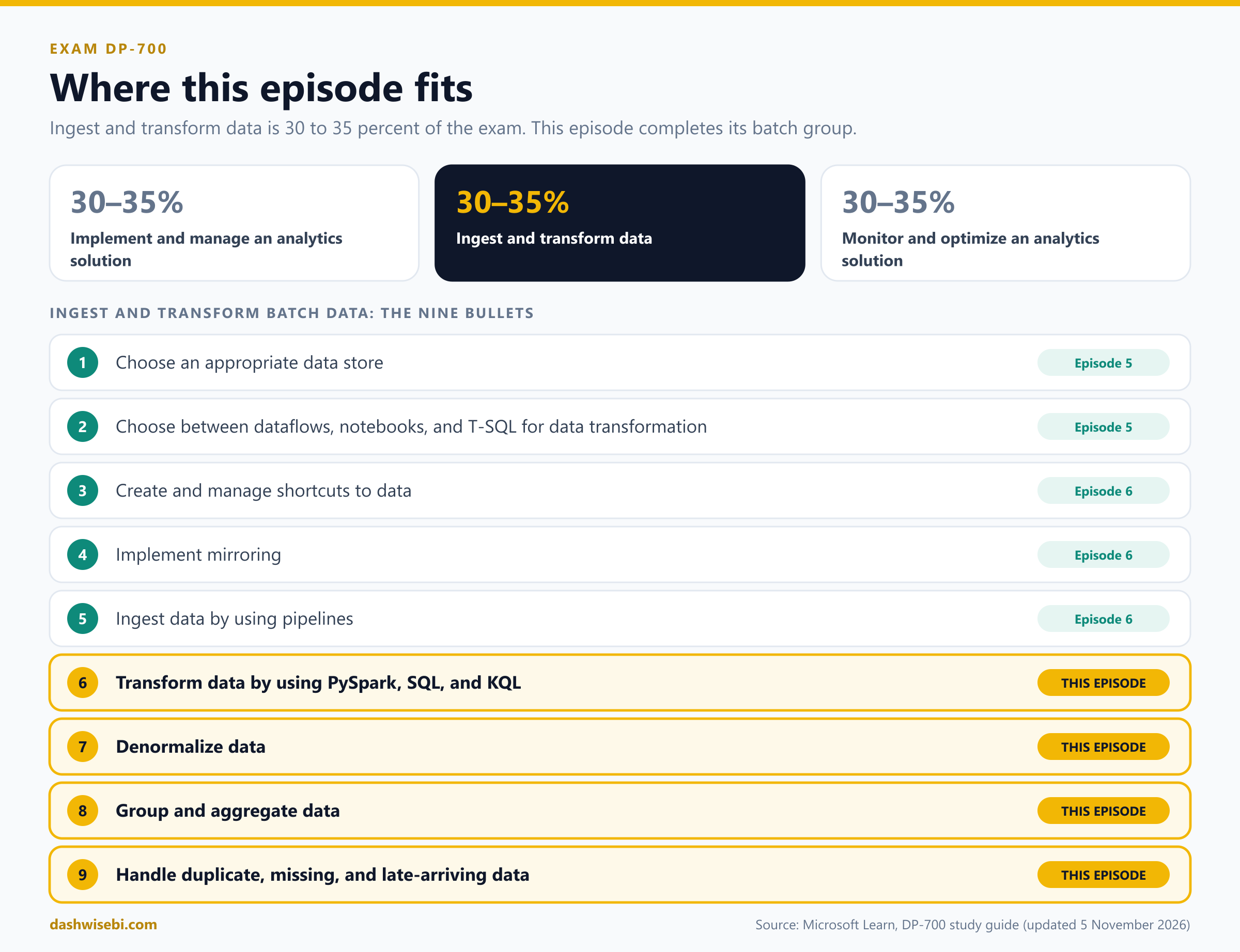
A note on wording. The study guide Microsoft updated on 5 November 2026 lists these as "Transform data by using PySpark, SQL, and KQL", "Denormalize data", "Group and aggregate data" and "Handle duplicate, missing, and late-arriving data", in the group Ingest and transform batch data. With this episode the whole batch group is covered. The streaming group (choosing a streaming engine, eventstreams, Spark structured streaming, KQL and windowing functions) comes next.
The companion demo: one dataset, three engines
This episode comes with three demo files. They all use the same small orders dataset, so you can watch one problem being solved three ways and compare the results row for row. Every code block in this post is taken from them. Download them from the table below (click a file name).
| File | Where it runs | What you need |
|---|---|---|
DP700_Ep7_Batch_Transformation_PySpark_Demo.ipynb | A Fabric notebook | A lakehouse attached as the default lakehouse, and Fabric Runtime 1.3 (Spark 3.5, Delta 3.2) or later. It creates all its own data, so there is nothing to upload. |
DP700_Ep7_Warehouse_TSQL_Demo.sql | A Warehouse, in a New SQL query | A Warehouse in the same workspace. Everything lives in the schema ep7, so it cannot clash with your own objects. |
DP700_Ep7_Eventhouse_KQL_Demo.kql | A KQL queryset on an Eventhouse | An Eventhouse (its KQL database is created with it). Put the cursor inside a block and press Shift+Enter. A block is the lines between blank lines. |
Run each file from top to bottom, one section at a time. In the SQL file, select a block and then run it. In the notebook, run the cells in order. A few blocks fail on purpose and are marked EXPECTED ERROR. Read the error message, because it is part of the lesson. The notebook tables are prefixed ep7_ and the SQL tables live in ep7, so you can clean up afterwards by dropping them.
What is planted in the data
The orders file is deliberately dirty. Every problem the exam asks about is in it once, so you can find it, fix it and check the fix:
| Problem | Where it is | Which section handles it |
|---|---|---|
| Exact duplicate row | Order 1005 appears twice, identical | 4 Duplicates |
| Two versions of one key | Order 1002: Pending first, Shipped (newer) at the end of the file | 4 Duplicates, upsert |
| Missing number | Order 1003 has no Qty | 1 typing traps, 4 Missing data |
| Placeholder and dirty text | Country is N/A, empty, " india " or india | 4 Missing data |
| Dimension that never arrives | Customer C999 and product P99 | 2 Unknown member |
| Dimension that arrives late | Customer C005 (orders 1009 and 1015) | 4 Late data |
| Batch 2, arriving on 2026-11-10 | 1002 becomes Delivered (an update). 1010 has an old order date (a late fact). 1015 is new. 1013 is delivered again unchanged (a repeat). A new Channel column appears (schema drift). | 4 Late data |
Where each part of the post lives in the demo files
| Post section | Notebook | T-SQL | KQL |
|---|---|---|---|
| 1 Transform | Sections 2, 3, 11 | Sections 1, 2, 10 | Sections 1, 2, 6 |
| 2 Denormalize | Sections 7, 10 | Sections 6, 9 | Sections 1, 6, 10 |
| 3 Group and aggregate | Section 8 | Section 7 | Section 7 |
| 4 Duplicates, missing, late | Sections 4, 5, 6, 9 | Sections 3, 4, 5, 8 | Sections 3, 4, 5, 8, 9 |
The big picture: three engines, three homes
In Episode 5 you learned to pick the tool that lives next to your data. Here is the same idea as a map. Each engine works on a different kind of store and has different powers.
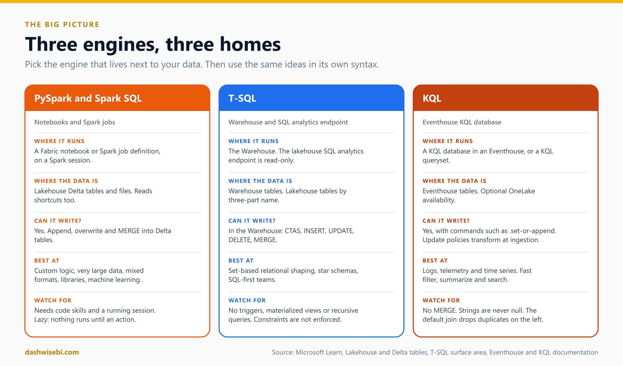
- PySpark and Spark SQL run in a notebook or a Spark job definition. They work mostly on lakehouse Delta tables and files, and can write back with append, overwrite and
MERGE. Fabric's lakehouse uses Delta Lake as its standard table format, so tables you write with Spark are readable by every other Fabric engine. - T-SQL runs in the Warehouse, where you can create tables and insert, update, delete and merge. It also runs on the lakehouse SQL analytics endpoint, but there it is read-only: you can create views, functions and procedures on top of the lakehouse tables, but you cannot create tables or change data.
- KQL runs in a KQL database in an Eventhouse. It is built for logs, telemetry and time series. It can read, and it can write with commands such as
.set-or-append, and update policies transform data as it arrives.
1. Transform data by using PySpark, SQL and KQL
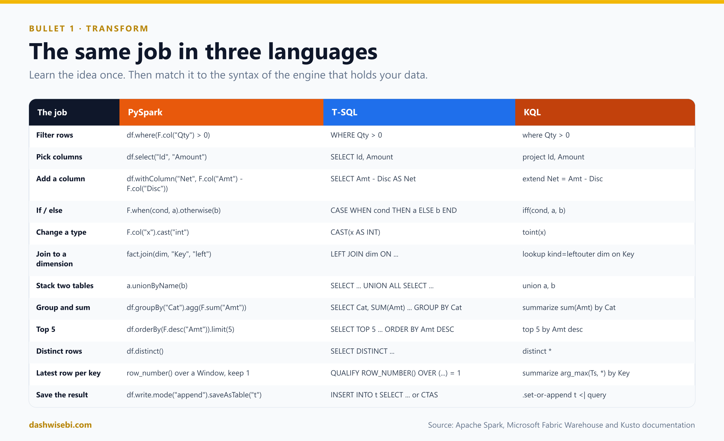
The first job is to get comfortable in all three languages. Start with this table. Every row is a task you do in almost every pipeline, written three ways.
PySpark in a notebook
A DataFrame is a distributed table. You describe a chain of transformations, and Spark runs them when you ask for a result, such as writing a table or showing rows. This is called lazy evaluation: withColumn, where and join build a plan, while write, show, count and collect are the actions that run it. The spark session is already created in a Fabric notebook.
from pyspark.sql import functions as F

raw = spark.read.format("csv").option("header", "true").load("Files/landing/orders/")

silver = (raw
    .withColumn("OrderDate", F.to_date("OrderDate", "yyyy-MM-dd"))
    .withColumn("Amount", F.col("Amount").cast("decimal(18,2)"))
    .withColumn("Country", F.upper(F.trim("Country")))
    .withColumn("Size", F.when(F.col("Amount") >= 1000, "Large").otherwise("Standard"))
    .where(F.col("OrderId").isNotNull()))

silver.write.mode("append").format("delta").saveAsTable("silver_orders")
The pieces to know:
- Read:
spark.readfor files,spark.tablefor a lakehouse table. Read a shortcut with a relative path, as you saw in Episode 6. - Shape:
select,where(orfilter),withColumn,drop,cast, andF.when(...).otherwise(...)for if-else. - Combine:
joinwith a type such as"inner"or"left".unionByNamestacks two DataFrames by column name, which is safer thanunion, which stacks by position. A small dimension can be broadcast so Spark sends it to every worker instead of shuffling the big table:fact.join(F.broadcast(dim), "ProductKey", "left"). - Write:
mode("append")adds rows,mode("overwrite")replaces the table, andsaveAsTableregisters it in the lakehouse. UseMERGE(section 4) for upserts. If a write adds new columns, setmergeSchemaso the table schema can grow.
From the demo: bronze, lazy evaluation and typing
The notebook lands the raw file into a bronze table exactly as it arrived. Nothing is typed or cleaned yet. Typing and cleaning happen in silver.
bronze_b1 = (
    spark.read
         .option("header", True)
         .csv(f"{LANDING_SPARK}/orders/orders_batch_01.csv")
         .withColumn("_source_file", F.col("_metadata.file_path"))
         .withColumn("_ingested_at", F.current_timestamp())
)

# Still nothing has executed. Look at the plan:
bronze_b1.explain()
spark.read.option("header", True).csv(...)withoutinferSchemareads every column as a string. That is intentional: bronze must never fail or silently change a value because a column looked like a number._metadata.file_pathis a hidden column that Spark adds when it reads files. Saving it as_source_file, together withcurrent_timestamp()as_ingested_at, gives every row its lineage: which file it came from and when it was loaded.- Nothing has run yet.
read,withColumnandselectonly build a plan, andexplain()prints that plan without executing it. This is lazy evaluation in action.
# An action triggers the job
print("Rows in batch 1:", bronze_b1.count())

bronze_b1.write.mode("overwrite").saveAsTable(f"{P}bronze_orders")
display(spark.table(f"{P}bronze_orders"))
count() is an action, so it triggers the first real job. saveAsTable is another action: it writes the Delta table. display shows the result in the notebook.
Then silver starts with typing and shaping:
orders_typed = (
    spark.table(f"{P}bronze_orders")
         .select(
             F.col("OrderID").cast("int").alias("OrderID"),
             F.trim("CustomerID").alias("CustomerID"),
             F.trim("ProductID").alias("ProductID"),
             F.to_date("OrderDate", "yyyy-MM-dd").alias("OrderDate"),
             F.col("Qty").cast("int").alias("Qty"),
             F.col("UnitPrice").cast("decimal(10,2)").alias("UnitPrice"),
             F.col("Country"),
             F.col("Status"),
             F.to_timestamp("ModifiedAt").alias("ModifiedAt"),
         )
         .withColumn("LineAmount", F.col("Qty") * F.col("UnitPrice"))
         .withColumn("OrderSize",
                     F.when(F.col("Qty") >= 5, "Large")
                      .when(F.col("Qty") >= 2, "Medium")
                      .when(F.col("Qty").isNotNull(), "Small")
                      .otherwise("Unknown"))
)

orders_typed.printSchema()
display(orders_typed.where(F.col("Status") != "Cancelled").orderBy("OrderID"))cast("int")turns the text"2"into the number 2. A value that cannot be converted, such as an empty string, becomesnullin Spark.to_date("OrderDate", "yyyy-MM-dd")needs the format that matches the text.cast("decimal(10,2)")keeps money exact instead of using a floating point type.LineAmountis derived withwithColumn. WhenQtyis null the product is null too, which is correct: we do not know the amount.F.when(...).when(...).otherwise(...)is evaluated top to bottom and the first match wins, so the order of the conditions matters. A nullQtydoes not satisfy>= 5or>= 2, so an explicitisNotNull()test is needed beforeotherwise("Unknown")to separate "Small" from "unknown".
union versus unionByName. This small test shows why the post recommends the second one:
a = spark.createDataFrame([(1, "India")], "OrderID INT, Country STRING")
b = spark.createDataFrame([("UK", 2)],    "Country STRING, OrderID INT")   # same columns, different order
c = spark.createDataFrame([(3, "USA", "Web")], "OrderID INT, Country STRING, Channel STRING")

print("union (positional): values land in the wrong columns")
a.union(b).show()

print("unionByName: matched by name")
a.unionByName(b).show()

print("unionByName(allowMissingColumns=True): Channel filled with null")
a.unionByName(c, allowMissingColumns=True).show()a.union(b)stacks by position. Framebhas the same columns in a different order, so the text"UK"lands in theOrderIDcolumn and the number 2 inCountry. Spark does not warn you.a.unionByName(b)matches by name, so each value lands in the right column.unionByName(c, allowMissingColumns=True)keeps going when one side has an extra column (Channel) and fills it withnullfor the rows that do not have it. You will need this for schema drift in section 4.
You can also mix in SQL. A %%sql cell, or spark.sql("..."), runs Spark SQL against the same tables:
%%sql
SELECT Category, SUM(Amount) AS Revenue
FROM gold_sales_wide
GROUP BY Category
From the demo: the same work in Spark SQL
A %%sql cell, or spark.sql(...), runs on the same Spark engine and sees the same tables. A temporary view created in PySpark is visible to SQL cells in the same session, which lets you move between languages in one notebook.
# Expose a clean batch to SQL
to_silver(spark.table(f"{P}bronze_orders")).createOrReplaceTempView("v_silver_candidates")

# spark.sql() from Python, e.g. to parameterise with f-strings
display(spark.sql(f"SELECT Status, COUNT(*) AS Orders FROM {P}silver_orders GROUP BY Status ORDER BY Status"))
The first line exposes the cleaned DataFrame as a view named v_silver_candidates. The second runs a SQL query from Python, where an f-string can parameterize the table name.
%%sql
WITH ranked AS (
    SELECT CAST(OrderID AS INT) AS OrderID, Status, ModifiedAt, _source_file,
           ROW_NUMBER() OVER (PARTITION BY OrderID ORDER BY CAST(ModifiedAt AS TIMESTAMP) DESC) AS rn
    FROM ep7_bronze_orders
)
SELECT * FROM ranked
WHERE OrderID IN (1002, 1013)
ORDER BY OrderID, rn
This is the latest-wins pattern as a common table expression: number the rows of each key by ModifiedAt descending. The bronze columns are still text, so ModifiedAt is cast to a timestamp inside the window. The query lists every row of orders 1002 and 1013 together with its rn, so you can see which row would survive: the one with rn = 1. Add WHERE rn = 1 to keep only that row. In a Fabric Warehouse you could write the filter directly with QUALIFY.
%%sql
MERGE INTO ep7_silver_orders AS t
USING v_silver_candidates AS s
   ON t.OrderID = s.OrderID
WHEN MATCHED AND s.ModifiedAt > t.ModifiedAt THEN UPDATE SET *
WHEN NOT MATCHED THEN INSERT *
This is the guarded upsert from section 4 in SQL. UPDATE SET * and INSERT * use every column of the source. The extra condition on the matched branch means an older or repeated row changes nothing.
%%sql
SELECT DATE_TRUNC('MONTH', OrderDate) AS Month,
       CategoryName,
       SUM(LineAmount)                AS Revenue,
       GROUPING_ID()                  AS GroupingLevel
FROM ep7_gold_sales_wide
WHERE Status <> 'Cancelled'
GROUP BY ROLLUP (DATE_TRUNC('MONTH', OrderDate), CategoryName)
ORDER BY Month NULLS LAST, CategoryName NULLS LAST
GROUP BY ROLLUP adds subtotal rows, and GROUPING_ID() returns a number that tells a subtotal row from a row where the column is genuinely null (0 means a detail row).
%%sql
DESCRIBE HISTORY ep7_silver_orders
first_merge_version = (spark.sql(f"DESCRIBE HISTORY {P}silver_orders")
.where("operation = 'MERGE'").agg(F.min("version")).first()[0])
display(spark.sql(f"""
SELECT 'v{first_merge_version} (after batch 1)' AS Snapshot, OrderID, Status, ModifiedAt
FROM {P}silver_orders VERSION AS OF {first_merge_version} WHERE OrderID = 1002
UNION ALL
SELECT 'current', OrderID, Status, ModifiedAt
FROM {P}silver_orders WHERE OrderID = 1002
"""))Every MERGE is a new version of the Delta table. DESCRIBE HISTORY lists the versions, and VERSION AS OF reads the table as it was. The last query shows order 1002 right after batch 1 (Shipped) next to its current state, which is useful when someone asks "what did this table say last week?".
T-SQL in the Warehouse
In the Warehouse you transform with set-based SQL. The usual tools are CTAS (CREATE TABLE ... AS SELECT), INSERT ... SELECT, UPDATE, DELETE, TRUNCATE TABLE, views, stored procedures and common table expressions (standard, sequential, and nested ones, which are in preview). MERGE is supported and generally available. Session-scoped #temp tables work too. Lakehouse tables in the same workspace can be read with a three-part name such as SilverLakehouse.dbo.orders.
INSERT INTO dbo.FactSales (OrderDate, ProductKey, Amount)
SELECT o.OrderDate, COALESCE(p.ProductKey, -1), o.Amount
FROM   SilverLakehouse.dbo.orders AS o
LEFT JOIN dbo.DimProduct AS p ON p.ProductId = o.ProductId;
Fabric supports some handy modern syntax: FROM-first queries, GROUP BY ALL and ORDER BY ALL without a column list, and QUALIFY to filter on a window function. It also has analytic functions such as MEDIAN, QUANTILE, APPROX_MEDIAN and APPROX_QUANTILE. Know the limits too. The following are not supported: triggers, materialized views, recursive queries, synonyms, CREATE USER and FOR XML. Primary key, unique and foreign key constraints can be added only as NOT ENFORCED, so they document intent but do not stop bad data. Column renames use sp_rename, and only a subset of ALTER TABLE is allowed.
From the demo: staging, typing traps and cross-database reads
The Warehouse script mirrors the notebook. It starts with a staging table where every column is VARCHAR, including empty strings and junk, which is the T-SQL version of bronze. In real life you would fill it with COPY INTO or OPENROWSET from OneLake. The demo inserts the same rows as the notebook's CSV file.
CREATE TABLE ep7.StagingOrders
(
    OrderID     VARCHAR(20),
    CustomerID  VARCHAR(20),
    ProductID   VARCHAR(20),
    OrderDate   VARCHAR(30),
    Qty         VARCHAR(20),
    UnitPrice   VARCHAR(20),
    Country     VARCHAR(50),
    Status      VARCHAR(20),
    ModifiedAt  VARCHAR(30),
    SourceFile  VARCHAR(100),
    LoadedAt    DATETIME2(6)
);
INSERT INTO ep7.StagingOrders
(OrderID, CustomerID, ProductID, OrderDate, Qty, UnitPrice, Country, Status, ModifiedAt, SourceFile, LoadedAt)
VALUES ('1001','C001','P01','2026-10-01','2' ,'25.00' ,'India' ,'Shipped' ,'2026-10-01 09:00:00','orders_batch_01.csv',SYSUTCDATETIME()),
('1002','C002','P02','2026-10-01','1' ,'120.00','India' ,'Pending' ,'2026-10-01 10:00:00','orders_batch_01.csv',SYSUTCDATETIME()),
('1003','C003','P03','2026-10-02','' ,'15.50' ,'USA' ,'Shipped' ,'2026-10-02 11:00:00','orders_batch_01.csv',SYSUTCDATETIME()),
-- ... 12 more rows: 15 in total, the same as orders_batch_01.csvA CTAS can also build small tables straight from a VALUES list, which is how the demo creates its source tables. The CAST calls fix the data types, because CTAS takes types from the query:
CREATE TABLE ep7.SrcCategory AS
SELECT CAST(CategoryKey AS INT) AS CategoryKey, CAST(CategoryName AS VARCHAR(50)) AS CategoryName
FROM (VALUES (1,'Electronics'),(2,'Home'),(3,'Office')) v(CategoryKey, CategoryName);
The typing trap. Spark turns an unparseable string into null. T-SQL does not always do that:
SELECT  TRY_CAST('' AS INT)                    AS EmptyToInt_Trap,      -- 0   (!)
        TRY_CAST(NULLIF(TRIM(''), '') AS INT)  AS EmptyToInt_Safe,      -- NULL
        TRY_CAST('N/A' AS INT)                 AS JunkToInt,            -- NULL
        TRY_CAST('' AS DATE)                   AS EmptyToDate_Trap;     -- 1900-01-01 (!)
TRY_CAST('' AS INT)returns 0, not null. An empty quantity would silently become a quantity of zero.- The same happens with dates:
TRY_CAST('' AS DATE)returns1900-01-01. - The safe pattern is
NULLIF(TRIM(x), '')first, which turns an empty (or blank) string intoNULL, and thenTRY_CAST. A real junk value such as'N/A'becomesNULLwithTRY_CASTalone.
The typed copy of staging uses that pattern, with TRIM on the text columns:
CREATE TABLE ep7.OrdersTyped AS
SELECT  TRY_CAST(OrderID AS INT)                                   AS OrderID,
        TRIM(CustomerID)                                           AS CustomerID,
        TRIM(ProductID)                                            AS ProductID,
        TRY_CAST(OrderDate AS DATE)                                AS OrderDate,
        TRY_CAST(NULLIF(TRIM(Qty), '') AS INT)                     AS Qty,
        TRY_CAST(UnitPrice AS DECIMAL(10,2))                       AS UnitPrice,
        Country,
        Status,
        TRY_CAST(ModifiedAt AS DATETIME2(6))                       AS ModifiedAt
FROM ep7.StagingOrders;
Reading the lakehouse tables from the Warehouse. Add the lakehouse to the Warehouse explorer, and use a three-part name (lakehouse.schema.table). The script keeps this block commented out, because you must replace <YourLakehouse> with your own lakehouse name first:
SELECT 'Lakehouse (Spark)' AS Source, COUNT(*) AS [Rows], SUM(LineAmount) AS Revenue
FROM <YourLakehouse>.dbo.ep7_silver_orders
UNION ALL
SELECT 'Warehouse (T-SQL)', COUNT(*), SUM(LineAmount)
FROM ep7.SilverOrders;

SELECT OrderID, Status, ModifiedAt FROM <YourLakehouse>.dbo.ep7_silver_orders
EXCEPT
SELECT OrderID, Status, ModifiedAt FROM ep7.SilverOrders;          -- expect 0 rows

-- >>> EXPECTED ERROR <<<  The lakehouse SQL analytics endpoint is READ-ONLY.
-- Write with Spark, a pipeline, a dataflow, or into a Warehouse instead.
INSERT INTO <YourLakehouse>.dbo.ep7_silver_orders (OrderID) VALUES (9999);
The first query compares row count and revenue between the Spark table and the Warehouse table. The EXCEPT query should return no rows when both agree. The last statement is the expected error: the lakehouse SQL analytics endpoint is read-only, so an INSERT fails. Write with Spark, a pipeline or a dataflow, or into a Warehouse.
KQL in an Eventhouse
KQL is a pipeline language. You start with a table and pass the rows through operators with the | character: where filters, project picks columns, extend adds columns, summarize aggregates, join and lookup combine tables, union stacks them, parse and extract pull values out of text, and mv-expand turns an array into rows.
let since = ago(7d);
RawLogs
| where Timestamp > since and isnotempty(Level)
| parse Message with "user=" User " action=" Action
| summarize Events = count(), Users = dcount(User) by Action, bin(Timestamp, 1h)
| order by Timestamp desc
A query only reads. To store a result you run a command that takes a query, for example .set-or-append (add to a table, create it if missing), .set-or-replace or .append:
.set-or-append HourlyActions <|
    RawLogs
    | where Timestamp > ago(1h)
    | summarize Events = count() by Action, bin(Timestamp, 1h)
To transform data as it arrives, attach an update policy to the target table (you met these in Episode 5). To keep a running aggregate or a deduplicated copy, use a materialized view (below). Two KQL traps appear in this section:
- The default join is
innerunique, notinner. It first removes duplicates from the left table on the join key, then matches. A join of events to a lookup can silently return fewer rows than you expect. Saykind=innerorkind=leftouterwhen you mean it. lookupis the dimension-enrichment operator. It is like a left outer join (the default kind) or an inner join, it does not repeat the key columns, and it assumes the left table is the large fact table and the right table is a small dimension. The right side is broadcast to every node, so if it is larger than several tens of megabytes the query fails.
From the demo: dimensions, an update policy and a join trap
In the Eventhouse you create dimensions with .set-or-replace. It creates the table if it does not exist and replaces its contents with the result of a query. A datatable supplies the rows inline. Customer C005 is missing on purpose:
.set-or-replace Customers <|
datatable(CustomerID:string, CustomerName:string, Segment:string, City:string)
[
    "C001", "Asha Traders",   "Retail",    "Pune",
    "C002", "Bright Office",  "Corporate", "Mumbai",
    "C003", "Campus Store",   "Education", "Nagpur",
    "C004", "Delta Supplies", "Retail",    "London"
]
Before any orders arrive, the demo creates the table and an update policy so every batch flows through it:
.create-merge table Orders (OrderID:int, CustomerID:string, ProductID:string, OrderDate:datetime, Qty:int, UnitPrice:real, Country:string, Status:string, ModifiedAt:datetime).create-merge table OrdersEnriched (OrderID:int, CustomerID:string, ProductID:string, OrderDate:datetime, Qty:int, UnitPrice:real, Country:string, Status:string, ModifiedAt:datetime, CustomerName:string, Segment:string).create-or-alter function with (folder="ep7", docstring="Enrich each new Orders batch with customer attributes") EnrichOrders()
{
Orders
| lookup kind=leftouter (Customers | project CustomerID, CustomerName, Segment) on CustomerID
| project OrderID, CustomerID, ProductID, OrderDate, Qty, UnitPrice, Country, Status, ModifiedAt, CustomerName, Segment
}.alter table OrdersEnriched policy update
@'[{"IsEnabled": true, "Source": "Orders", "Query": "EnrichOrders()", "IsTransactional": false}]'.create-merge tablecreates the table, or adds any missing columns if it exists.OrdersEnrichedis the target and has two extra columns for the customer.EnrichOrders()is a stored function. Inside an update policy, the nameOrdersmeans only the batch being ingested, not the whole table. It useslookup kind=leftouterto copy the customer attributes onto each new row.- The policy says: when data lands in
Orders, runEnrichOrders()and store the result inOrdersEnriched. Create the policy before you ingest, or the first batches will not be enriched.
The join trap, measured. This query counts the rows from four ways of joining the latest orders to the customers:
union
    (OrdersLatest | join Customers on CustomerID                  | count | extend JoinKind = "1 default (innerunique)"),
    (OrdersLatest | join kind=inner Customers on CustomerID       | count | extend JoinKind = "2 kind=inner"),
    (OrdersLatest | join kind=leftouter Customers on CustomerID   | count | extend JoinKind = "3 kind=leftouter"),
    (OrdersLatest | lookup kind=leftouter Customers on CustomerID | count | extend JoinKind = "4 lookup leftouter")
| project JoinKind, Rows = Count
| order by JoinKind asc- The default join (
innerunique) removes duplicate keys on the left side first. With orders on the left, it keeps only one order per customer, so the count is far lower than the real number of orders. kind=innerkeeps every matching order.kind=leftouterandlookup kind=leftouteralso keep the orders whose customer is missing. Always writekind=explicitly.
2. Denormalize data
A normalized model stores each fact once and splits attributes across many tables, which is good for writing. A denormalized model copies attributes into the table that is read, which is good for reporting. In an analytics platform you normally normalize at the source and denormalize on the way to the gold layer.
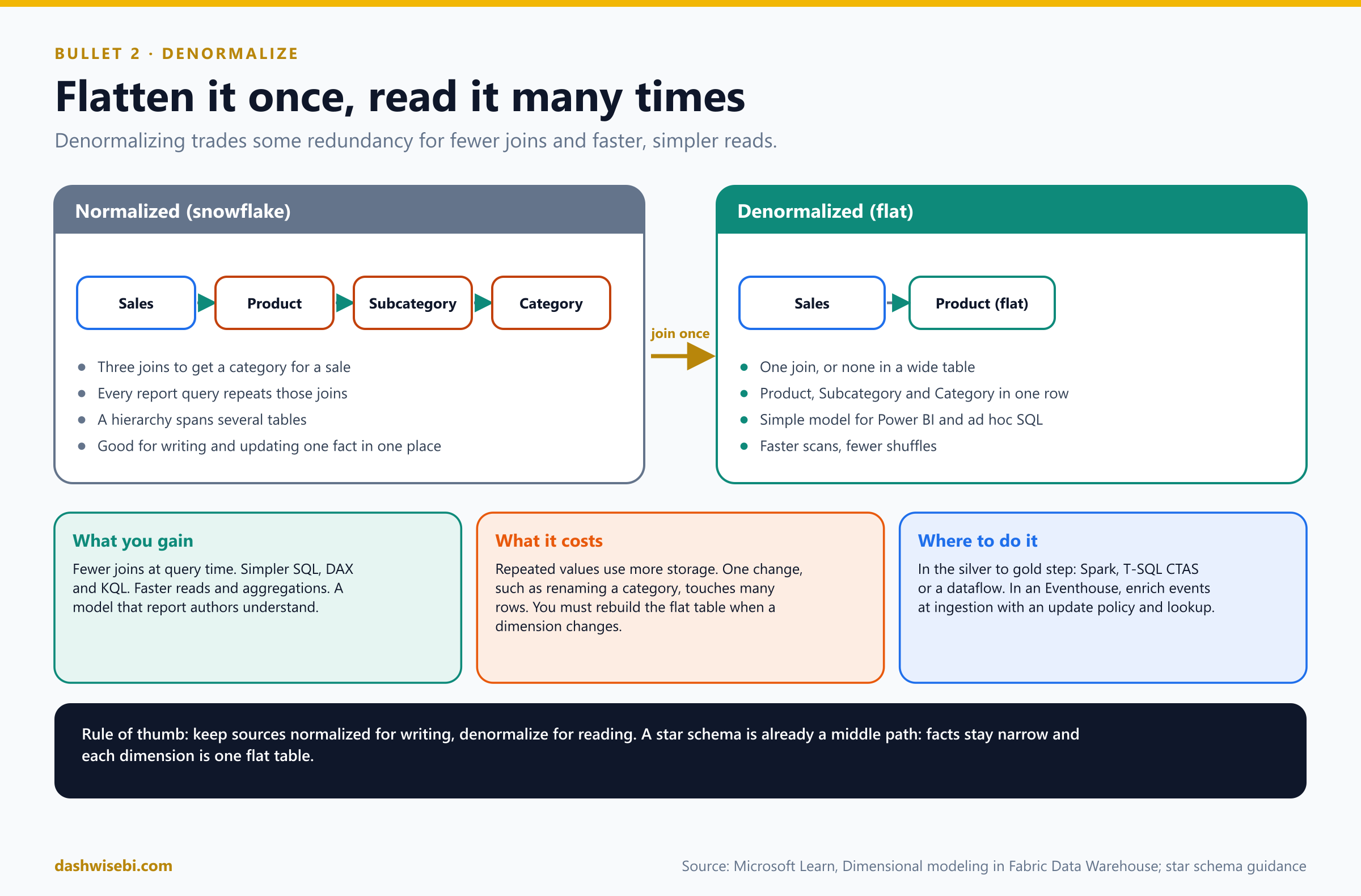
What it looks like
- Flatten a snowflake dimension. Join Product, Subcategory and Category into one
DimProducttable that holds all three levels. This is the most common exam example, and it is how a star schema is built from a snowflake. You can read the reasons in our PL-300 data model episode: fewer tables, a hierarchy in one table, shorter filter paths. - Build a wide table. Join facts to several dimensions once and store the result, so a report or a notebook reads one table with no joins.
- Flatten nested data. JSON from an API or an event often has structs and arrays. Turn them into columns and rows before analysis.
- Enrich events at ingestion. In an Eventhouse, copy dimension attributes onto each event with an update policy that uses
lookup, so queries never need to join.
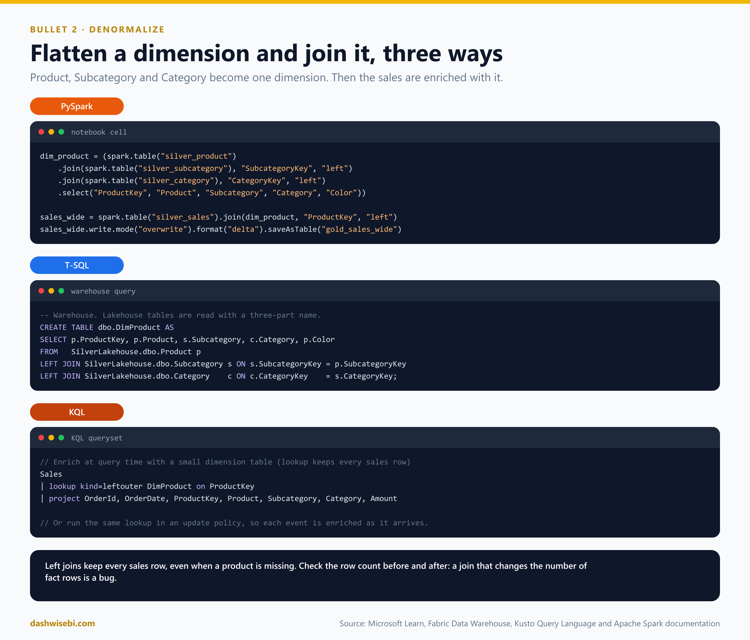
From the demo: flatten the snowflake and build a wide table
The demo's source is a snowflake: Category, then Subcategory, then Product, plus Customer. The goal is a flat DimProduct with an Unknown member (key -1) for facts whose product does not exist.
PySpark
def build_dim_product():
    dim = (spark.table(f"{P}src_product")
           .join(spark.table(f"{P}src_subcategory"), "SubcategoryKey", "left")
           .join(spark.table(f"{P}src_category"), "CategoryKey", "left")
           .select("ProductKey", "ProductID", "ProductName", "SubcategoryName", "CategoryName", "ListPrice"))
    unknown = spark.createDataFrame([(-1, "N/A", "Unknown", "Unknown", "Unknown", None)], dim.schema)
    dim.unionByName(unknown).write.mode("overwrite").saveAsTable(f"{P}dim_product")


def build_dim_customer():
    dim = spark.table(f"{P}src_customer")
    unknown = spark.createDataFrame([(-1, "N/A", "Unknown", "Unknown", "Unknown")], dim.schema)
    dim.unionByName(unknown).write.mode("overwrite").saveAsTable(f"{P}dim_customer")


build_dim_product()
build_dim_customer()
display(spark.table(f"{P}dim_product").orderBy("ProductKey"))- Joining on the column name (
"SubcategoryKey") keeps a single copy of the key column."left"keeps every product even if a subcategory is missing. - The Unknown row is built with the schema of the dimension (
dim.schema) and added withunionByName.mode("overwrite")rebuilds the table, so running it again after the source changes is safe.
T-SQL, with a CTAS that does the same in one statement:
CREATE TABLE ep7.DimProduct AS
SELECT  p.ProductKey, p.ProductID, p.ProductName, s.SubcategoryName, c.CategoryName, p.ListPrice
FROM ep7.SrcProduct p
LEFT JOIN ep7.SrcSubcategory s ON s.SubcategoryKey = p.SubcategoryKey
LEFT JOIN ep7.SrcCategory    c ON c.CategoryKey    = s.CategoryKey
UNION ALL
SELECT -1, 'N/A', 'Unknown', 'Unknown', 'Unknown', NULL;KQL, where lookup is the dimension-enrichment join and a one-row datatable adds the Unknown member:
.set-or-replace DimProduct <|
Product
| lookup kind=leftouter Subcategory on SubcategoryKey
| lookup kind=leftouter Category on CategoryKey
| project ProductKey, ProductID, ProductName, SubcategoryName, CategoryName, ListPrice
| union (datatable(ProductKey:int, ProductID:string, ProductName:string, SubcategoryName:string, CategoryName:string, ListPrice:real)
         [ -1, "N/A", "Unknown", "Unknown", "Unknown", real(null) ])
The KQL comment in the demo says it plainly: lookup broadcasts the small right side. Always say kind=leftouter, so that a missing subcategory does not remove the product.
The row explosion trap, with a check you can run
If the dimension key is not unique, the join multiplies fact rows. The keys are not enforced, so the database will not stop it. The demo adds a second copy of product P01 and compares row counts:
bad_dim = spark.table(f"{P}dim_product").unionByName(
    spark.table(f"{P}dim_product").where("ProductID = 'P01'"))   # P01 now appears twice

silver = spark.table(f"{P}silver_orders")
print("Fact rows:", silver.count(),
      "| after join to bad dim:", silver.join(bad_dim, "ProductID", "left").count())

def assert_unique(df, key):
    dupes = df.groupBy(key).count().where("count > 1")
    n = dupes.count()
    if n:
        display(dupes)
        raise ValueError(f"{n} duplicate value(s) in key '{key}'")
    print(f"OK: '{key}' is unique")

assert_unique(spark.table(f"{P}dim_product"), "ProductID")
try:
    assert_unique(bad_dim, "ProductID")
except ValueError as e:
    print("Caught:", e)
WITH bad_dim AS
(
SELECT * FROM ep7.DimProduct
UNION ALL
SELECT * FROM ep7.DimProduct WHERE ProductID = 'P01' -- P01 now appears twice
)
SELECT (SELECT COUNT(*) FROM ep7.SilverOrders) AS FactRows,
(SELECT COUNT(*) FROM ep7.SilverOrders f LEFT JOIN bad_dim d ON d.ProductID = f.ProductID) AS RowsAfterJoin;
-- Uniqueness check to run in ETL (keys are NOT ENFORCED): should return nothing
SELECT ProductID, COUNT(*) AS Cnt FROM ep7.DimProduct GROUP BY ProductID HAVING COUNT(*) > 1;- The "fact rows" count and the "rows after join" count should match. With the doubled
P01, the second number is larger, and every revenue total that touches P01 is inflated. assert_uniquein the notebook, and the lastGROUP BY ... HAVING COUNT(*) > 1query in SQL, are the check to put in your ETL. It should return nothing. In the notebook it raises an error, which stops the pipeline before bad numbers reach a report.
The wide gold table
Now join the fact to the dimensions once, and store the result so reports read one table. In all three versions the rule is the same: start from the fact, use a left join, and map a missing dimension to -1 and "Unknown", so that no sale is ever dropped.
def build_gold_sales_wide():
    f = spark.table(f"{P}silver_orders").alias("f")
    p = spark.table(f"{P}dim_product").alias("p")
    c = spark.table(f"{P}dim_customer").alias("c")
    wide = (
        f.join(F.broadcast(p), F.col("f.ProductID") == F.col("p.ProductID"), "left")
         .join(F.broadcast(c), F.col("f.CustomerID") == F.col("c.CustomerID"), "left")
         .select(
             "f.OrderID", "f.OrderDate", "f.Status", "f.Country", "f.Qty", "f.UnitPrice", "f.LineAmount",
             F.coalesce("p.ProductKey", F.lit(-1)).alias("ProductKey"),
             F.coalesce("p.ProductName", F.lit("Unknown")).alias("ProductName"),
             F.coalesce("p.CategoryName", F.lit("Unknown")).alias("CategoryName"),
             F.coalesce("c.CustomerKey", F.lit(-1)).alias("CustomerKey"),
             F.coalesce("c.CustomerName", F.lit("Unknown")).alias("CustomerName"),
             F.coalesce("c.Segment", F.lit("Unknown")).alias("Segment"),
             F.col("f.CustomerID").alias("SourceCustomerID"),
             F.col("f.ProductID").alias("SourceProductID"),
         )
    )
    wide.write.mode("overwrite").option("overwriteSchema", True).saveAsTable(f"{P}gold_sales_wide")


build_gold_sales_wide()
gold = spark.table(f"{P}gold_sales_wide")
print("Silver rows:", spark.table(f"{P}silver_orders").count(), "| Gold rows:", gold.count())

print("Rows mapped to the Unknown member:")
display(gold.where("ProductKey = -1 OR CustomerKey = -1")
.select("OrderID", "SourceCustomerID", "CustomerKey", "SourceProductID", "ProductKey"))F.broadcast(p)andF.broadcast(c)tell Spark to send the small dimensions to every worker, so the big fact table is not shuffled.F.coalesce("p.ProductKey", F.lit(-1))returns the first non-null value: the real key if the join matched, otherwise-1.- The original keys are kept as
SourceCustomerIDandSourceProductID, so you can see why a row is Unknown and repair it later.
In T-SQL the demo wraps the build in a stored procedure, so it can be rerun after a late dimension arrives (section 4):
CREATE PROCEDURE ep7.usp_BuildGold
AS
BEGIN
    DROP TABLE IF EXISTS ep7.DimCustomer;
    CREATE TABLE ep7.DimCustomer AS
    SELECT CustomerKey, CustomerID, CustomerName, Segment, City FROM ep7.SrcCustomer
    UNION ALL
    SELECT -1, 'N/A', 'Unknown', 'Unknown', 'Unknown';

    DROP TABLE IF EXISTS ep7.FactSalesWide;
    CREATE TABLE ep7.FactSalesWide AS
    SELECT  f.OrderID, f.OrderDate, f.Status, f.Country, f.Qty, f.UnitPrice, f.LineAmount,
            COALESCE(p.ProductKey, -1)           AS ProductKey,
            COALESCE(p.ProductName, 'Unknown')   AS ProductName,
            COALESCE(p.CategoryName, 'Unknown')  AS CategoryName,
            COALESCE(c.CustomerKey, -1)          AS CustomerKey,
            COALESCE(c.CustomerName, 'Unknown')  AS CustomerName,
            COALESCE(c.Segment, 'Unknown')       AS Segment,
            f.CustomerID                         AS SourceCustomerID,
            f.ProductID                          AS SourceProductID
    FROM ep7.SilverOrders f
    LEFT JOIN ep7.DimProduct  p ON p.ProductID  = f.ProductID
    LEFT JOIN ep7.DimCustomer c ON c.CustomerID = f.CustomerID;
END;
GO
EXEC ep7.usp_BuildGold;The procedure rebuilds both tables with DROP TABLE IF EXISTS and CTAS each time. The rows that end up on the Unknown member are order 1006 (customer C999), 1007 (product P99) and 1009 (customer C005, who has not arrived yet). You can list them with the check query in the script:
SELECT OrderID, SourceCustomerID, CustomerKey, SourceProductID, ProductKey
FROM ep7.FactSalesWide
WHERE CustomerKey = -1 OR ProductKey = -1
ORDER BY OrderID;
In KQL the equivalent is a stored function, so the join happens at query time:
.create-or-alter function with (folder="ep7", docstring="Wide sales: latest orders + product + customer") SalesWide()
{
    OrdersLatest
    | extend LineAmount = Qty * UnitPrice
    | lookup kind=leftouter (DimProduct | project ProductID, ProductKey, ProductName, CategoryName) on ProductID
    | lookup kind=leftouter (Customers | project CustomerID, CustomerName, Segment) on CustomerID
    | extend ProductKey   = coalesce(ProductKey, int(-1)),
             ProductName  = iff(isempty(ProductName),  "Unknown", ProductName),
             CategoryName = iff(isempty(CategoryName), "Unknown", CategoryName),
             CustomerName = iff(isempty(CustomerName), "Unknown", CustomerName),
             Segment      = iff(isempty(Segment),      "Unknown", Segment)
}- Left outer lookups return empty strings (not nulls) for text columns when there is no match. That is why the function uses
iff(isempty(...), "Unknown", ...)for the strings. - For the integer
ProductKeythe missing value is a real null, socoalesce(ProductKey, int(-1))works. This is the same trap you will meet again in the missing-data part:coalesce()does not replace empty strings.
Flatten nested JSON
In Spark use explode to turn an array into one row per element, and dot notation to reach into a struct. In KQL use mv-expand on a dynamic column.
orders = spark.read.json("Files/landing/orders_json/")
items = (orders
    .select("OrderId", F.col("Customer.Id").alias("CustomerId"), F.explode("Items").alias("item"))
    .select("OrderId", "CustomerId", "item.Sku", "item.Qty", "item.Price"))
Orders
| mv-expand item = Items
| project OrderId, CustomerId = tostring(Customer.Id), Sku = tostring(item.Sku),
Qty = toint(item.Qty), Price = todouble(item.Price)From the demo: JSON in all three engines
The demo's JSON has three orders. Order 2001 has two line items, order 2002 has one, and order 2003 has none. That last one shows the difference between dropping and keeping empty arrays.
PySpark
orders_j = spark.read.json(f"{LANDING_SPARK}/orders_json/")
orders_j.printSchema()

flat = (orders_j
        .select("OrderID",
                F.to_date("OrderDate").alias("OrderDate"),
                F.col("Customer.CustomerID").alias("CustomerID"),     # dot notation into a struct
                F.col("Customer.City").alias("City"),
                F.explode("Items").alias("item"))                     # one row per line item
        .select("*", "item.*").drop("item")
        .withColumn("LineAmount", F.col("Qty") * F.col("UnitPrice")))

display(flat)

print("explode rows:      ", orders_j.select(F.explode("Items")).count())
print("explode_outer rows:", orders_j.select(F.explode_outer("Items")).count(), "(keeps order 2003)")F.col("Customer.CustomerID")uses dot notation to reach into a struct.F.explode("Items")gives one row per element, and thenselect("*", "item.*")turns the element's fields into columns.- The two counts at the end show the difference:
explodedrops order 2003 because its array is empty, andexplode_outerkeeps it with nulls.
T-SQL uses OPENJSON to read the document and CROSS APPLY to expand the array:
DECLARE @orders VARCHAR(8000) = '[
  {"OrderID":2001,"OrderDate":"2026-11-01","Customer":{"CustomerID":"C001","City":"Pune"},
   "Items":[{"ProductID":"P01","Qty":2,"UnitPrice":25.0},{"ProductID":"P03","Qty":1,"UnitPrice":15.5}]},
  {"OrderID":2002,"OrderDate":"2026-11-02","Customer":{"CustomerID":"C002","City":"Mumbai"},
   "Items":[{"ProductID":"P02","Qty":1,"UnitPrice":120.0}]},
  {"OrderID":2003,"OrderDate":"2026-11-03","Customer":{"CustomerID":"C003","City":"Nagpur"},
   "Items":[]}
]';

SELECT  o.OrderID, o.OrderDate, o.CustomerID, o.City,
        i.ProductID, i.Qty, i.UnitPrice, i.Qty * i.UnitPrice AS LineAmount
FROM OPENJSON(@orders)
     WITH (OrderID    INT          '$.OrderID',
           OrderDate  DATE         '$.OrderDate',
           CustomerID VARCHAR(10)  '$.Customer.CustomerID',     -- "dot notation" into the struct
           City       VARCHAR(30)  '$.Customer.City',
           Items      NVARCHAR(MAX) '$.Items' AS JSON) o           -- AS JSON requires NVARCHAR(MAX)
CROSS APPLY OPENJSON(o.Items)
     WITH (ProductID VARCHAR(10), Qty INT, UnitPrice DECIMAL(10,2)) i;
SELECT 'CROSS APPLY' AS Mode, COUNT(*) AS [Rows]
FROM OPENJSON(@orders) WITH (Items NVARCHAR(MAX) '$.Items' AS JSON) o
CROSS APPLY OPENJSON(o.Items) i
UNION ALL
SELECT 'OUTER APPLY', COUNT(*)
FROM OPENJSON(@orders) WITH (Items NVARCHAR(MAX) '$.Items' AS JSON) o
OUTER APPLY OPENJSON(o.Items) i; -- 3 vs 4 rows- The
WITHclause maps JSON paths to typed columns.'$.Customer.CustomerID'is the path syntax for reaching into an object. Items NVARCHAR(MAX) '$.Items' AS JSONkeeps the array as JSON text for the next step. TheAS JSONoption requiresNVARCHAR(MAX).CROSS APPLY OPENJSON(o.Items)behaves likeexplode(order 2003 disappears).OUTER APPLYbehaves likeexplode_outer(order 2003 stays, with nulls). The final query counts the rows: 3 forCROSS APPLYand 4 forOUTER APPLY.- For a JSON file in OneLake, read it with
OPENROWSET(BULK '<path to the .jsonl file>')and then useCROSS APPLY OPENJSONexactly as above.
KQL
.set-or-replace OrdersJson <|
datatable(OrderID:int, OrderDate:datetime, Customer:dynamic, Items:dynamic)
[
    2001, datetime(2026-11-01), dynamic({"CustomerID":"C001","City":"Pune"}),
          dynamic([{"ProductID":"P01","Qty":2,"UnitPrice":25.0},{"ProductID":"P03","Qty":1,"UnitPrice":15.5}]),
    2002, datetime(2026-11-02), dynamic({"CustomerID":"C002","City":"Mumbai"}),
          dynamic([{"ProductID":"P02","Qty":1,"UnitPrice":120.0}]),
    2003, datetime(2026-11-03), dynamic({"CustomerID":"C003","City":"Nagpur"}),
          dynamic([])
]
OrdersJson
| mv-expand Item = Items
| project OrderID, OrderDate,
CustomerID = tostring(Customer.CustomerID), // dot notation into the property bag
City = tostring(Customer.City),
ProductID = tostring(Item.ProductID),
Qty = toint(Item.Qty),
UnitPrice = todouble(Item.UnitPrice)
| extend LineAmount = Qty * UnitPrice- A
dynamiccolumn holds JSON.Customer.CustomerIDis dot notation into the property bag, and you convert the value withtostring(),toint()ortodouble(). mv-expand Item = Itemsgives one row per array element. Likeexplode, it drops the row whose array is empty.
To keep order 2003, as explode_outer would, turn the empty array into an array with one null before expanding it:
union
    (OrdersJson | mv-expand Items | count | extend Mode = "mv-expand (like explode)"),
    (OrdersJson | extend Items = iff(array_length(Items) == 0, dynamic([null]), Items)
                | mv-expand Items | count | extend Mode = "empty -> [null] (like explode_outer)")
| project Mode, Rows = Count
The same demo also shows how to turn log-like text into columns with parse and extract:
datatable(Line:string)
[
    "2026-11-10 09:00:00 ORDER 1002 status=Delivered channel=Web",
    "2026-11-10 09:05:00 ORDER 1010 status=Shipped channel=Store"
]
| parse Line with EventTime:datetime " ORDER " OrderID:int " status=" Status:string " channel=" Channel:string
| extend StatusViaExtract = extract(@"status=(\w+)", 1, Line)
parse reads the pieces between the literal words and gives them types (EventTime:datetime, OrderID:int). extract pulls one value with a regular expression, here the word after status=.
Trade-offs and traps
- It is a trade. You gain simpler queries and faster reads, and you pay in storage, in update effort (change a category name and many rows change) and in the need to rebuild the flat table when a dimension changes.
- A join can multiply rows. If the dimension has two rows for one key, every matching fact row appears twice and your totals double. Check that the dimension key is unique and compare row counts before and after the join. Fabric does not enforce keys for you.
- Use a left join from the fact. It keeps every fact row. Where the dimension is missing, fill the key with the Unknown member (
-1), as you learned in Episode 5. - Mind history. For a slowly changing dimension (type 2), a denormalized fact should carry the attribute that was true at the time of the event. Join on the key and on the validity range:
SELECT f.OrderId, f.Amount, d.Segment
FROM   dbo.FactSales AS f
JOIN   dbo.DimCustomer AS d
  ON   d.CustomerId = f.CustomerId
AND f.OrderDate >= d.ValidFrom AND f.OrderDate < d.ValidTo;- Do not denormalize the source system. Transactional databases stay normalized. Denormalize in the layer built for reading.
- Update policies need the dimension to be there. If the dimension row arrives after the event, the lookup at ingestion finds nothing. More on this in section 4.
3. Group and aggregate data
To aggregate is to collapse many rows into fewer, with a measure for each group. The first decision is the grain: what does one output row represent? Here it is one row per month and category. Once the grain is clear, the syntax is straightforward in all three engines.
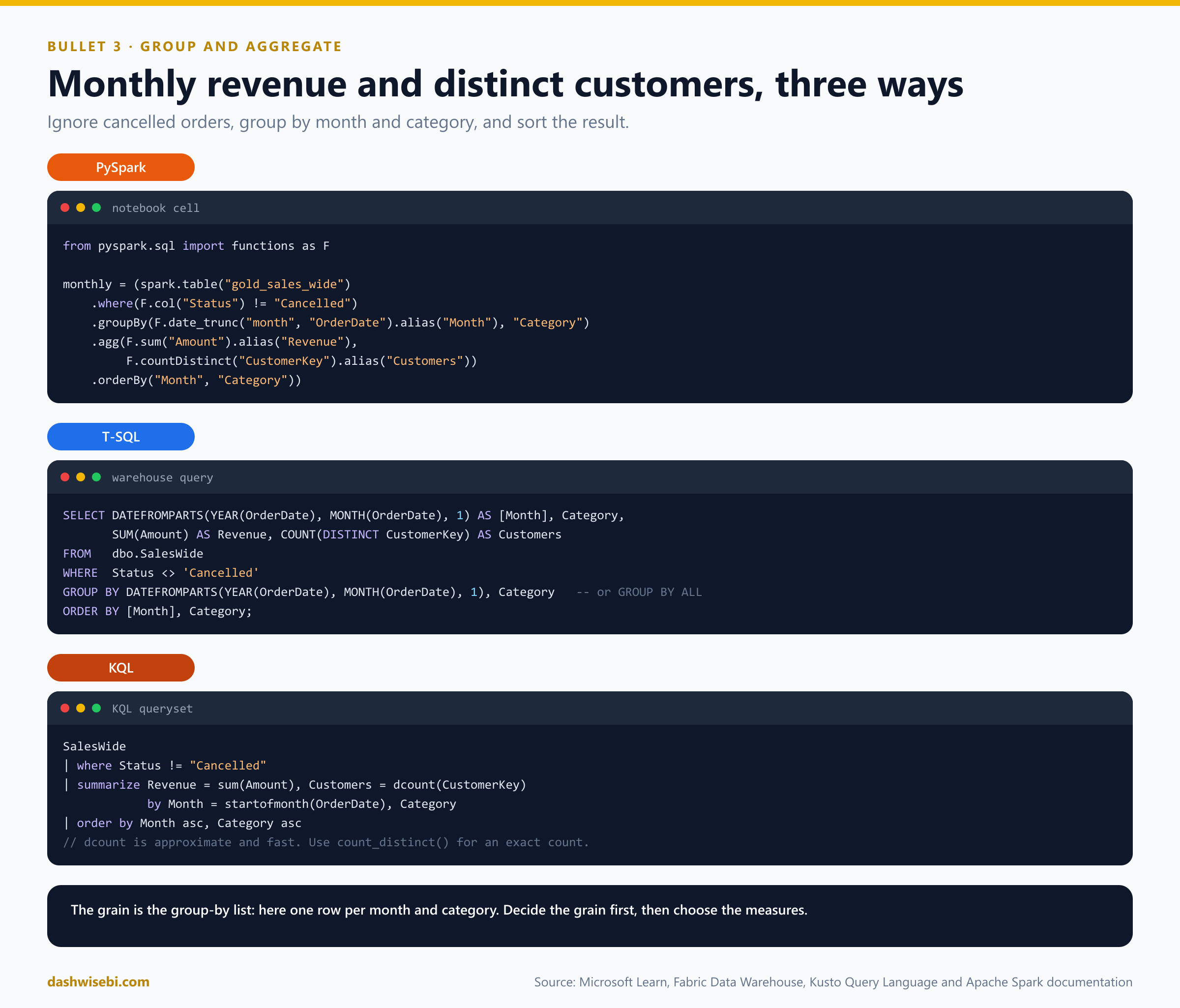
PySpark
Use groupBy(...).agg(...) with functions such as F.sum, F.count, F.countDistinct, F.avg, F.min, F.max, F.collect_list and F.approx_count_distinct. Add rollup and cube for subtotals, and pivot to turn values into columns. Window functions keep every row and add a calculation across related rows: ranks, running totals, previous and next values.
from pyspark.sql import Window

sales.rollup("Category", "Subcategory").agg(F.sum("Amount").alias("Revenue"))
sales.groupBy("Category").pivot("Year", [2025, 2026]).sum("Amount")

w = (Window.partitionBy("Category").orderBy("Month")
           .rowsBetween(Window.unboundedPreceding, Window.currentRow))
monthly.withColumn("RunningRevenue", F.sum("Revenue").over(w))
From the demo: aggregates in PySpark
The grain is one row per month and category, and cancelled orders are excluded first. The demo uses the wide gold table from section 2:
sales = (spark.table(f"{P}gold_sales_wide")
              .where("Status <> 'Cancelled'")
              .withColumn("Month", F.trunc("OrderDate", "month")))

monthly = (sales.groupBy("Month", "CategoryName")
                .agg(F.sum("LineAmount").alias("Revenue"),
                     F.count("*").alias("Rows"),
                     F.count("Qty").alias("RowsWithQty"),           # count(col) skips nulls
                     F.countDistinct("OrderID").alias("Orders"),
                     F.approx_count_distinct("CustomerKey").alias("ApproxCustomers"),
                     F.avg("LineAmount").alias("AvgLine"),
                     F.min("OrderDate").alias("FirstOrder"),
                     F.max("OrderDate").alias("LastOrder"),
                     F.collect_set("ProductName").alias("Products"))
                .orderBy("Month", "CategoryName"))

display(monthly)
F.trunc("OrderDate", "month")turns a date into the first day of its month, which becomes the grouping column.F.count("*")counts rows.F.count("Qty")counts only rows whereQtyis not null. Putting both side by side (RowsandRowsWithQty) makes the missing quantity visible.countDistinctis exact.approx_count_distinctis faster and uses less memory, with a small error.collect_setgathers the distinct product names into an array.
Subtotals and pivots. rollup adds a subtotal per month and a grand total. cube adds every combination of the columns. grouping_id() says which level a row is:
display(sales.rollup("Month", "CategoryName")
             .agg(F.sum("LineAmount").alias("Revenue"), F.grouping_id().alias("GroupingLevel"))
             .orderBy(F.col("Month").asc_nulls_last(), F.col("CategoryName").asc_nulls_last()))
display(sales.cube("Month", "Segment")
.agg(F.sum("LineAmount").alias("Revenue"))
.orderBy(F.col("Month").asc_nulls_last(), F.col("Segment").asc_nulls_last()))pivot turns the category values into columns. Listing the values yourself saves Spark an extra scan to discover them:
categories = ["Electronics", "Home", "Office", "Unknown"]   # listing values avoids an extra scan
display(sales.groupBy("Month").pivot("CategoryName", categories).agg(F.sum("LineAmount")).orderBy("Month"))
Window functions keep every row and add a calculation over related rows, unlike groupBy, which collapses them:
daily = sales.groupBy("OrderDate").agg(F.sum("LineAmount").alias("Revenue"))

w_running = Window.orderBy("OrderDate").rowsBetween(Window.unboundedPreceding, Window.currentRow)
w_moving3 = Window.orderBy("OrderDate").rowsBetween(-2, Window.currentRow)

display(daily.withColumn("RunningRevenue", F.sum("Revenue").over(w_running))
             .withColumn("Moving3DayAvg", F.round(F.avg("Revenue").over(w_moving3), 2))
             .orderBy("OrderDate"))
w_rank = Window.partitionBy("CategoryName").orderBy(F.col("Revenue").desc())
display(sales.groupBy("CategoryName", "ProductName").agg(F.sum("LineAmount").alias("Revenue"))
.withColumn("RankInCategory", F.dense_rank().over(w_rank))
.orderBy("CategoryName", "RankInCategory"))rowsBetween(Window.unboundedPreceding, Window.currentRow)sums from the first day up to the current one, which is a running total.rowsBetween(-2, Window.currentRow)averages the current day and the two before it, which is a 3-day moving average.dense_rank()numbers products by revenue within each category and does not skip numbers when there are ties (rank()would).
Empty input. This pitfall shows up when a filter removes every row:
empty = sales.where("1 = 0")
print("agg without groupBy:", empty.agg(F.sum("LineAmount")).collect())
print("agg with groupBy:   ", empty.groupBy("Month").agg(F.sum("LineAmount")).collect())
The aggregate without groupBy returns one row holding a null. With groupBy it returns no rows. A downstream step that expects at least one row works in the first case and breaks in the second.
T-SQL
Use GROUP BY, with HAVING to filter groups after they are built (WHERE filters rows before). In the Warehouse, GROUP BY ALL groups by every non-aggregated column in the select list. Window functions use OVER (PARTITION BY ... ORDER BY ...).
SELECT Category, [Month], Revenue,
       SUM(Revenue) OVER (PARTITION BY Category ORDER BY [Month]
                          ROWS BETWEEN UNBOUNDED PRECEDING AND CURRENT ROW) AS RunningRevenue
FROM   dbo.MonthlyRevenue;
From the demo: aggregates in the Warehouse
The same grain, built with a CTAS so the result is stored as a gold table:
CREATE TABLE ep7.MonthlyRevenue AS
SELECT  DATEFROMPARTS(YEAR(OrderDate), MONTH(OrderDate), 1) AS [Month],
        CategoryName,
        SUM(LineAmount)               AS Revenue,
        COUNT(*)                      AS [Rows],
        COUNT(Qty)                    AS RowsWithQty,
        COUNT(DISTINCT OrderID)       AS Orders,
        COUNT(DISTINCT CustomerKey)   AS Customers,
        AVG(LineAmount)               AS AvgLine
FROM ep7.FactSalesWide
WHERE Status <> 'Cancelled'                      -- WHERE filters rows BEFORE grouping
GROUP BY DATEFROMPARTS(YEAR(OrderDate), MONTH(OrderDate), 1), CategoryName;WHEREremoves the cancelled rows before grouping.COUNT(*)counts rows andCOUNT(Qty)skips nulls, exactly as in Spark.- The grouping expression is repeated in
GROUP BY, because the alias[Month]is not available there.
HAVING filters the groups after aggregation:
SELECT CategoryName, SUM(LineAmount) AS Revenue
FROM ep7.FactSalesWide
WHERE Status <> 'Cancelled'
GROUP BY CategoryName
HAVING SUM(LineAmount) > 150;
Subtotals with ROLLUP. GROUPING_ID tells a subtotal row apart from a row where the category is really null:
WITH sales AS
(
    SELECT DATEFROMPARTS(YEAR(OrderDate), MONTH(OrderDate), 1) AS [Month], CategoryName, LineAmount
    FROM ep7.FactSalesWide
    WHERE Status <> 'Cancelled'
)
SELECT  [Month], CategoryName,
        SUM(LineAmount)                   AS Revenue,
        GROUPING_ID([Month], CategoryName) AS GroupingLevel     -- 0 detail, 1 month subtotal, 3 grand total
FROM sales
GROUP BY ROLLUP ([Month], CategoryName)
ORDER BY GroupingLevel, [Month], CategoryName;
The grouping level is 0 for a detail row, 1 for a month subtotal and 3 for the grand total, so the ORDER BY GroupingLevel puts details first and the grand total last.
Window functions: a running total, a 3-day moving average and a rank:
WITH daily AS
(
    SELECT OrderDate, SUM(LineAmount) AS Revenue
    FROM ep7.FactSalesWide
    WHERE Status <> 'Cancelled'
    GROUP BY OrderDate
)
SELECT  OrderDate, Revenue,
        SUM(Revenue) OVER (ORDER BY OrderDate ROWS UNBOUNDED PRECEDING)              AS RunningRevenue,
        AVG(Revenue) OVER (ORDER BY OrderDate ROWS BETWEEN 2 PRECEDING AND CURRENT ROW) AS Moving3DayAvg
FROM daily
ORDER BY OrderDate;

SELECT  CategoryName, ProductName, SUM(LineAmount) AS Revenue,
        DENSE_RANK() OVER (PARTITION BY CategoryName ORDER BY SUM(LineAmount) DESC) AS RankInCategory
FROM ep7.FactSalesWide
WHERE Status <> 'Cancelled'
GROUP BY CategoryName, ProductName
ORDER BY CategoryName, RankInCategory;
DENSE_RANK() OVER (PARTITION BY CategoryName ORDER BY SUM(LineAmount) DESC) ranks the products inside each category. Note that the window function is evaluated after the grouping, which is why it can use SUM(LineAmount).
Percentiles, approximate and exact:
SELECT  CategoryName,
        APPROX_PERCENTILE_CONT(0.5) WITHIN GROUP (ORDER BY LineAmount) AS ApproxMedianLine
FROM ep7.FactSalesWide
WHERE Status <> 'Cancelled'
GROUP BY CategoryName;

SELECT DISTINCT CategoryName,
       PERCENTILE_CONT(0.5) WITHIN GROUP (ORDER BY LineAmount) OVER (PARTITION BY CategoryName) AS ExactMedianLine
FROM ep7.FactSalesWide
WHERE Status <> 'Cancelled';APPROX_PERCENTILE_CONTis an aggregate function, fast and suitable for big tables. Use it when a small error is acceptable.PERCENTILE_CONT ... OVER (PARTITION BY ...)is exact, but it is a window function, so it repeats the value on every row and needsSELECT DISTINCTto give one row per category.
Empty input: no GROUP BY returns one row with null, and with GROUP BY it returns zero rows, the same as in Spark.
SELECT SUM(LineAmount) AS NoGroupBy FROM ep7.FactSalesWide WHERE 1 = 0;
SELECT CategoryName, SUM(LineAmount) AS WithGroupBy FROM ep7.FactSalesWide WHERE 1 = 0 GROUP BY CategoryName;
KQL
summarize is the aggregation operator. Group by a column, or by a time bucket made with bin(). Useful aggregates are count(), countif(), dcount(), count_distinct(), sum(), sumif(), avg(), percentile(), make_list(), make_set(), arg_max() and take_any(). For a running total, sort the rows and use row_cumsum():
MonthlyRevenue
| sort by Category asc, Month asc
| extend RunningRevenue = row_cumsum(Revenue, Category != prev(Category))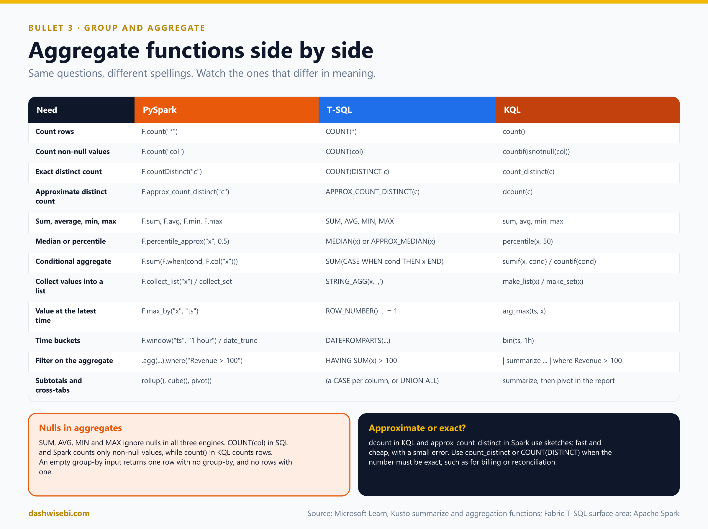
From the demo: aggregates in KQL
First, one summarize with the common aggregation functions:
SalesWide
| where Status != "Cancelled"
| summarize Revenue     = sum(LineAmount),
            Rows        = count(),
            RowsWithQty = countif(isnotnull(Qty)),
            Orders      = dcount(OrderID),           // approximate (HyperLogLog)
            OrdersExact = count_distinct(OrderID),   // exact, more expensive
            AvgLine     = avg(LineAmount),
            P50Line     = percentile(LineAmount, 50),
            Products    = make_set(ProductName)
         by Month = startofmonth(OrderDate), CategoryName
| order by Month asc, CategoryName asc
Orders = dcount(OrderID)is approximate (HyperLogLog), andOrdersExact = count_distinct(OrderID)is exact but more expensive.Rows = count()counts rows.RowsWithQty = countif(isnotnull(Qty))counts non-null values, the KQL way of writingCOUNT(Qty).percentile(LineAmount, 50)is the median.make_setcollects the distinct product names.startofmonth(OrderDate)builds the month.
Conditional aggregates compute several measures in one pass, instead of filtering the table repeatedly:
SalesWide
| summarize ShippedRevenue = sumif(LineAmount, Status in ("Shipped", "Delivered")),
            PendingOrders  = countif(Status == "Pending"),
            CancelledRows  = countif(Status == "Cancelled")
         by CategoryName
Daily totals, a running total and a day-over-day change. bin(OrderDate, 1d) rounds to the day. The rows must be sorted before row_cumsum() and prev() work as expected:
SalesWide
| where Status != "Cancelled"
| summarize Revenue = sum(LineAmount) by Day = bin(OrderDate, 1d)
| order by Day asc
| extend RunningRevenue = row_cumsum(Revenue),
         DeltaVsPrevDay = Revenue - prev(Revenue)
Top product per category. arg_max(Revenue, ProductName) returns the product name from the row with the highest revenue in each category:
SalesWide
| where Status != "Cancelled"
| summarize Revenue = sum(LineAmount) by CategoryName, ProductName
| summarize arg_max(Revenue, ProductName) by CategoryName
High-cardinality groups. When there are very many groups, hint.strategy=shuffle spreads the aggregation across nodes:
Orders
| summarize hint.strategy=shuffle Rows = count() by CustomerID
Pre-aggregate with a materialized view. The view built in section 4 aggregates across batches. Read it like a table:
ChangesPerDay
| order by Day asc
A query only reads, so to store a gold aggregate you use a command:
.set-or-replace GoldDailyRevenue <|
SalesWide
| where Status != "Cancelled"
| summarize Revenue = sum(LineAmount) by OrderDate = bin(OrderDate, 1d)
Things that trip people up
- Nulls.
SUM,AVG,MINandMAXskip null values.COUNT(col)in SQL and Spark counts non-null values, butcount()in KQL counts rows, so count non-null values withcountif(isnotnull(col)). - Empty input. With no group-by, an aggregate over no rows returns one row (counts and sums are 0, other results are null). With a group-by it returns no rows.
- Approximate versus exact.
dcount()in KQL andapprox_count_distinctin Spark use sketches: fast, cheap, small error. Usecount_distinct(),countDistinctorCOUNT(DISTINCT)when the number must be exact. - High-cardinality groups. In KQL, a
summarizewith a very large number of groups can be spread across nodes with the shuffle hint,summarize hint.strategy=shuffle .... Spark does the equivalent shuffle for you on agroupBy. - Pre-aggregate what you read often. A gold aggregate table, or a KQL materialized view, answers common questions without scanning the raw data every time. A materialized view always returns fresh results: it combines the already-aggregated part with the newest records that are not yet processed. Query the materialized part only, with
materialized_view("Name"), when you accept a little staleness for speed. - Update policy or materialized view? Update policies run on each ingestion batch, so they can only aggregate within one batch. For real aggregation across batches, use a materialized view.
4. Handle duplicate, missing and late-arriving data
Real data is messy. Sources resend records, leave gaps, and deliver things after you thought the day was finished. The exam tests whether you can name the problem and choose the pattern. Start with duplicates.
Duplicates
There are three kinds, and they need different fixes:
- Exact copies. Every column is the same, for example because a file was loaded twice. Remove them with
DISTINCT,dropDuplicates()ordistinct *. - Several versions of one key. The same order arrives again with a newer
ModifiedAt. You want the latest. A plain distinct will not remove them, because the rows differ. - Repeated deliveries of an event. A stream or API delivers each event at least once, so the same event ID can appear twice. Keep one.
First find them. Group by the key and keep groups with more than one row:
df.groupBy("OrderId").count().where("count > 1")

SELECT OrderId, COUNT(*) AS Copies FROM dbo.StagingOrders GROUP BY OrderId HAVING COUNT(*) > 1;

Orders | summarize Copies = count() by OrderId | where Copies > 1
Then remove them:
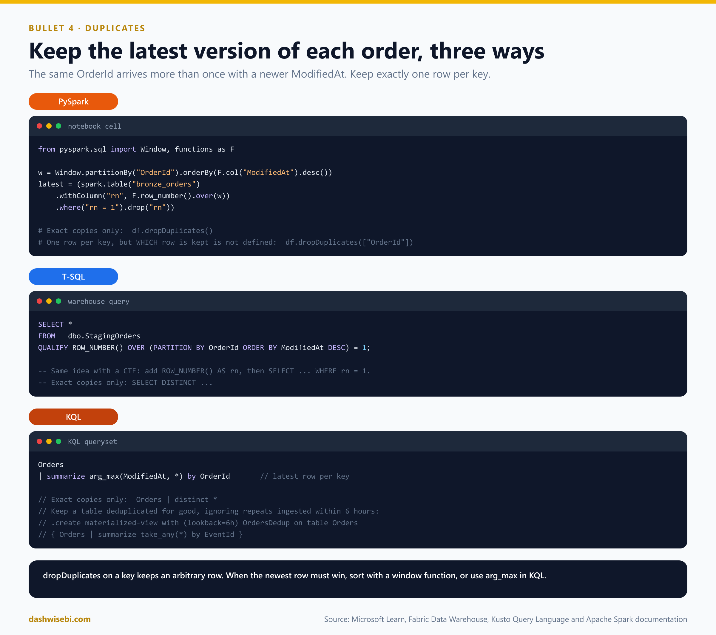
- Latest per key uses a window function. Number the rows in each key by
ModifiedAtdescending and keep number 1:row_number()in Spark,ROW_NUMBER()withQUALIFY(or a CTE) in T-SQL, andsummarize arg_max(ModifiedAt, *) by OrderIdin KQL. dropDuplicates(["OrderId"])keeps an arbitrary row. Spark does not promise which one survives, so it is fine for exact copies and wrong when the newest version must win.distinct()compares all columns, whiledropDuplicates(subset)compares only the columns you list.- Constraints will not save you. In the Warehouse, primary and unique keys are
NOT ENFORCED, and a Delta table has no enforced key either. Deduplication is your ETL's job.
From the demo: find and remove duplicates
The orders file has 15 rows: 1005 twice (exact copies), and two versions of 1002. Work through the same steps in each engine.
PySpark: detect, then see what each tool does:
display(
    orders_typed.groupBy("OrderID")
                .agg(F.count("*").alias("Copies"),
                     F.countDistinct("ModifiedAt").alias("Versions"))
                .where("Copies > 1")
)
print("Rows:", orders_typed.count(), "| after distinct():", orders_typed.distinct().count())
display(orders_typed.distinct().where("OrderID IN (1002, 1005)").orderBy("OrderID", "ModifiedAt"))- The first query lists keys that occur more than once, with the number of copies and distinct versions. 1005 has 2 copies and 1 version, and 1002 has 2 copies and 2 versions.
distinct()compares all columns, so 15 rows become 14: the identical 1005 collapses, and both versions of 1002 survive.
display(orders_typed.dropDuplicates(["OrderID"]).where("OrderID = 1002")
                    .select("OrderID", "Status", "ModifiedAt"))
This is the dropDuplicates trap. Keeping "one row per OrderID" without an ordering returns an arbitrary row, so the stale Pending version of 1002 can survive. Even when it happens to pick the right one, that is luck.
w_latest = Window.partitionBy("OrderID").orderBy(F.col("ModifiedAt").desc())

orders_dedup = (orders_typed
                .withColumn("rn", F.row_number().over(w_latest))
                .where("rn = 1")
                .drop("rn"))

print("Rows after latest-wins dedup:", orders_dedup.count())
display(orders_dedup.where("OrderID IN (1002, 1005)").select("OrderID", "Status", "ModifiedAt"))
The window version is deterministic: partition by the business key, order by ModifiedAt descending, keep rn = 1. The result has 13 rows, and order 1002 is Shipped.
T-SQL: the same four steps. Detect uses HAVING, because the filter is on a group:
SELECT  OrderID,
        COUNT(*)                   AS Copies,
        COUNT(DISTINCT ModifiedAt) AS Versions
FROM ep7.OrdersTyped
GROUP BY OrderID
HAVING COUNT(*) > 1;
SELECT DISTINCT * FROM ep7.OrdersTyped WHERE OrderID IN (1002, 1005) ORDER BY OrderID, ModifiedAt;WITH ranked AS
(
SELECT *,
ROW_NUMBER() OVER (PARTITION BY OrderID ORDER BY ModifiedAt DESC) AS rn
FROM ep7.OrdersTyped
)
SELECT OrderID, Status, ModifiedAt
FROM ranked
WHERE rn = 1 AND OrderID IN (1002, 1005);The CTE with ROW_NUMBER() works everywhere. The version with QUALIFY filters on the window function without a CTE:
SELECT OrderID, Status, ModifiedAt
FROM ep7.OrdersTyped
WHERE OrderID IN (1002, 1005)
QUALIFY ROW_NUMBER() OVER (PARTITION BY OrderID ORDER BY ModifiedAt DESC) = 1;
The script notes that if your Warehouse returns a syntax error on QUALIFY, the feature is not enabled for you yet, and the CTE version is what the rest of the script relies on.
KQL: the demo loads the file twice on purpose, to simulate a pipeline retry (the protected form, with an ingest-by tag, comes in the upsert part below). The four sources then show four different row counts:
union
    (Orders                              | summarize Rows = count() | extend Source = "1 Orders (raw)"),
    (OrdersDedup                         | summarize Rows = count() | extend Source = "2 OrdersDedup (take_any)"),
    (materialized_view("OrdersDedup")    | summarize Rows = count() | extend Source = "3 materialized part only"),
    (OrdersLatest                        | summarize Rows = count() | extend Source = "4 OrdersLatest (arg_max)")
| project Source, Rows
| order by Source ascOrders(raw) has 30 rows: 15 twice. The deduplicated viewOrdersDeduphas 14, andOrdersLatesthas 13, one per order.- Querying a materialized view by name returns the materialized part plus the records not yet processed, so it is always fresh.
materialized_view("OrdersDedup")reads only the materialized part, which is faster but can lag right after an ingestion.
Query-time versions of detect and dedup:
Orders
| summarize Copies = count(), Versions = dcount(ModifiedAt) by OrderID
| where Copies > 1
| order by OrderID asc
Orders
| summarize arg_max(ModifiedAt, *) by OrderID
| where OrderID in (1002, 1005)
| project OrderID, Status, ModifiedAtOrders
| distinct *
| where OrderID in (1002, 1005)
| project OrderID, Status, ModifiedAt
| order by OrderID asc, ModifiedAt ascarg_max(ModifiedAt, *) is KQL's row_number() = 1: it returns the whole row with the latest ModifiedAt for each OrderID. distinct * compares all columns, so both versions of 1002 stay, as in the other engines.
Keep it clean with an upsert
A better design is to make the load idempotent: running it twice gives the same result as running it once. The standard tool is MERGE, which updates rows that match the key and inserts rows that do not.
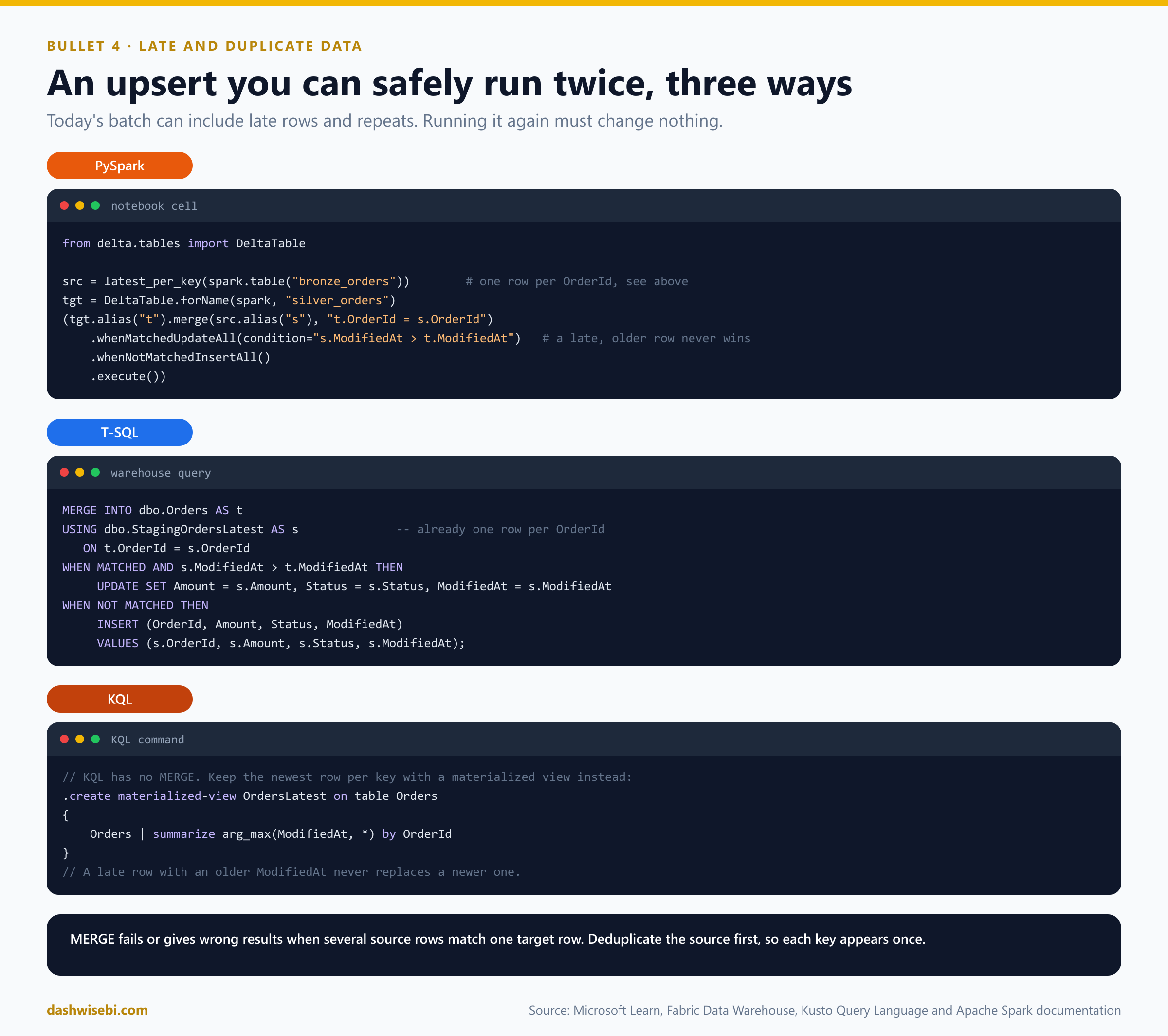
- The source must have one row per key. If several source rows match one target row, the merge is ambiguous and Delta can fail. Deduplicate the source first, as in the previous step.
- Guard against old rows. Adding
s.ModifiedAt > t.ModifiedAtto the matched clause stops a late, older version from overwriting a newer one. - Insert-only merge removes repeated events. With only a "when not matched, insert" clause, a record that already exists is ignored. Add a date-range condition so Delta does not scan the whole table:
(tgt.alias("t")
    .merge(src.alias("s"),
           "t.EventId = s.EventId AND t.EventDate >= current_date() - INTERVAL 7 DAYS")
    .whenNotMatchedInsertAll()
.execute())- KQL has no MERGE. To keep the latest row per key, use a materialized view with
arg_max. To drop repeated deliveries, use a materialized view withtake_any(*)grouped by the event ID, and give it a lookback so it deduplicates only against records ingested in a recent window, for example 6 hours:
.create materialized-view with (lookback=6h) EventsDedup on table Events
{
    Events | summarize take_any(*) by EventId
}
KQL can also stop duplicate loads at ingestion: tag an ingestion with an ingest-by: tag and use the ingestIfNotExists property, so a batch that was already ingested is skipped. And a materialized view can be created over another materialized view when the source one is a deduplication view (take_any(*)).
From the demo: build silver with a guarded upsert
PySpark. The cleanup steps are packaged into one reusable function, to_silver(), and the upsert into upsert_silver():
def to_silver(bronze_df):
    """Type, standardize, dedup (latest wins) and flag missing values."""
    w = Window.partitionBy("OrderID").orderBy(F.col("ModifiedAt").desc())
    return (
        bronze_df.select(
            F.col("OrderID").cast("int").alias("OrderID"),
            F.trim("CustomerID").alias("CustomerID"),
            F.trim("ProductID").alias("ProductID"),
            F.to_date("OrderDate", "yyyy-MM-dd").alias("OrderDate"),
            F.col("Qty").cast("int").alias("Qty"),
            F.col("UnitPrice").cast("decimal(10,2)").alias("UnitPrice"),
            F.when(F.upper(F.trim("Country")).isin(PLACEHOLDERS), F.lit(None))
             .when(F.length(F.trim("Country")) <= 3, F.upper(F.trim("Country")))
             .otherwise(F.initcap(F.trim("Country"))).alias("Country"),
            F.trim("Status").alias("Status"),
            F.to_timestamp("ModifiedAt").alias("ModifiedAt"),
        )
        .withColumn("rn", F.row_number().over(w)).where("rn = 1").drop("rn")
        .withColumn("LineAmount", F.col("Qty") * F.col("UnitPrice"))
        .withColumn("QtyMissing", F.col("Qty").isNull())
        .fillna({"Country": "Unknown"})
    )


def upsert_silver(source_df):
    target = DeltaTable.forName(spark, f"{P}silver_orders")
    (target.alias("t")
           .merge(source_df.alias("s"), "t.OrderID = s.OrderID")
           .whenMatchedUpdateAll(condition="s.ModifiedAt > t.ModifiedAt")
           .whenNotMatchedInsertAll()
           .execute())


def fingerprint(table):
    """Row count + order-independent checksum, used to prove idempotency."""
    df = spark.table(table)
    return df.select(F.count("*").alias("rows"),
                     F.sum(F.xxhash64(*df.columns).cast("decimal(38,0)")).alias("checksum")).first()


def last_merge_metrics(table):
    return (DeltaTable.forName(spark, table).history(1)
            .select("version", "operation", "operationMetrics.numSourceRows",
"operationMetrics.numTargetRowsInserted", "operationMetrics.numTargetRowsUpdated"))to_silver()types, standardizes, deduplicates (latest wins) and flags missing values. Because it is a function, batch 2 later goes through exactly the same logic.upsert_silver()is a DeltaMERGE. The conditions.ModifiedAt > t.ModifiedAton the matched branch is the guard: an older or repeated row can never overwrite a newer one. That guard is what makes the load idempotent.fingerprint()returns the row count and an order-independent checksum of all rows (xxhash64summed). Two equal fingerprints mean the table did not change.last_merge_metrics()reads the numbers of rows inserted and updated by the last merge from the Delta history.
silver_b1 = to_silver(spark.table(f"{P}bronze_orders"))

# Create the empty silver table with the right schema, then load it via MERGE
if not spark.catalog.tableExists(f"{P}silver_orders"):
    silver_b1.limit(0).write.saveAsTable(f"{P}silver_orders")

upsert_silver(silver_b1)

display(last_merge_metrics(f"{P}silver_orders"))
display(spark.table(f"{P}silver_orders").orderBy("OrderID"))
The silver table is created empty with the right schema, then loaded by the same MERGE that later loads will use. The first run inserts 13 rows.
The failing merge. This block merges the un-deduplicated rows, with no guard, into a scratch copy:
spark.table(f"{P}silver_orders").write.mode("overwrite").saveAsTable(f"{P}scratch_merge_demo")

dirty_source = orders_typed.withColumn("QtyMissing", F.col("Qty").isNull()).drop("OrderSize")

try:
    (DeltaTable.forName(spark, f"{P}scratch_merge_demo").alias("t")
        .merge(dirty_source.alias("s"), "t.OrderID = s.OrderID")
        .whenMatchedUpdateAll()          # no guard, no dedup
        .whenNotMatchedInsertAll()
        .execute())
    print("MERGE succeeded (unexpected)")
except Exception as e:
    print("MERGE failed as expected:\n", str(e).splitlines()[0][:300])
It fails, because several source rows (two 1002s and two 1005s) match one target row and Delta cannot tell which should win. The fix is the one the function already applies: deduplicate the source to one row per key first.
Prove idempotency. Run the same load again and compare:
before = fingerprint(f"{P}silver_orders")
upsert_silver(to_silver(spark.table(f"{P}bronze_orders")))   # rerun the same batch
after = fingerprint(f"{P}silver_orders")

print("Before:", before)
print("After: ", after)
print("Idempotent:", before == after)
display(last_merge_metrics(f"{P}silver_orders"))
If the fingerprints are equal, the second run changed nothing, and the merge metrics show 0 rows inserted and 0 updated.
T-SQL. The twin of to_silver() is a view:
CREATE VIEW ep7.vw_SilverCandidates AS
WITH typed AS
(
    SELECT  TRY_CAST(OrderID AS INT)                         AS OrderID,
            TRIM(CustomerID)                                 AS CustomerID,
            TRIM(ProductID)                                  AS ProductID,
            TRY_CAST(OrderDate AS DATE)                      AS OrderDate,
            TRY_CAST(NULLIF(TRIM(Qty), '') AS INT)           AS Qty,
            TRY_CAST(UnitPrice AS DECIMAL(10,2))             AS UnitPrice,
            CASE WHEN Country IS NULL
                   OR UPPER(TRIM(Country)) IN ('', 'N/A', 'NA', 'NULL', '-', 'UNKNOWN') THEN 'Unknown'
                 WHEN LEN(TRIM(Country)) <= 3 THEN UPPER(TRIM(Country))
                 ELSE UPPER(LEFT(TRIM(Country), 1)) + LOWER(SUBSTRING(TRIM(Country), 2, 100))
            END                                              AS Country,
            TRIM(Status)                                     AS Status,
            TRY_CAST(ModifiedAt AS DATETIME2(6))             AS ModifiedAt
    FROM ep7.StagingOrders
),
ranked AS
(
    SELECT *, ROW_NUMBER() OVER (PARTITION BY OrderID ORDER BY ModifiedAt DESC) AS rn
    FROM typed
)
SELECT  OrderID, CustomerID, ProductID, OrderDate, Qty, UnitPrice, Country, Status, ModifiedAt,
        CAST(Qty * UnitPrice AS DECIMAL(18,2))               AS LineAmount,
        CAST(CASE WHEN Qty IS NULL THEN 1 ELSE 0 END AS BIT) AS QtyMissing
FROM ranked
WHERE rn = 1;
It types the columns (with NULLIF(TRIM(...), '') for the quantity), standardizes the country, keeps the latest row per order, and adds LineAmount and a QtyMissing flag. Then the silver table, with a primary key that can only be NOT ENFORCED:
CREATE TABLE ep7.SilverOrders
(
    OrderID     INT           NOT NULL,
    CustomerID  VARCHAR(20),
    ProductID   VARCHAR(20),
    OrderDate   DATE,
    Qty         INT,
    UnitPrice   DECIMAL(10,2),
    Country     VARCHAR(50),
    Status      VARCHAR(20),
    ModifiedAt  DATETIME2(6),
    LineAmount  DECIMAL(18,2),
    QtyMissing  BIT
);
ALTER TABLE ep7.SilverOrders ADD CONSTRAINT PK_SilverOrders PRIMARY KEY NONCLUSTERED (OrderID) NOT ENFORCED;
The demo proves that NOT ENFORCED means not enforced: duplicate keys go straight in.
CREATE TABLE ep7.PkDemo (OrderID INT NOT NULL, Note VARCHAR(20));
ALTER TABLE ep7.PkDemo ADD CONSTRAINT PK_PkDemo PRIMARY KEY NONCLUSTERED (OrderID) NOT ENFORCED;
INSERT INTO ep7.PkDemo VALUES (1, 'first'), (1, 'duplicate!');
SELECT * FROM ep7.PkDemo;          -- 2 rows with the same "primary key"
The last query returns two rows with the same "primary key". Keep this in mind for the exam: the constraint documents intent and helps the optimizer, but your ETL must check uniqueness.
The guarded upsert, which should leave 13 rows with 1002 = Shipped:
MERGE ep7.SilverOrders AS t
USING ep7.vw_SilverCandidates AS s
   ON t.OrderID = s.OrderID
WHEN MATCHED AND s.ModifiedAt > t.ModifiedAt THEN
    UPDATE SET CustomerID = s.CustomerID, ProductID = s.ProductID, OrderDate = s.OrderDate,
               Qty = s.Qty, UnitPrice = s.UnitPrice, Country = s.Country, Status = s.Status,
               ModifiedAt = s.ModifiedAt, LineAmount = s.LineAmount, QtyMissing = s.QtyMissing
WHEN NOT MATCHED BY TARGET THEN
    INSERT (OrderID, CustomerID, ProductID, OrderDate, Qty, UnitPrice, Country, Status, ModifiedAt, LineAmount, QtyMissing)
    VALUES (s.OrderID, s.CustomerID, s.ProductID, s.OrderDate, s.Qty, s.UnitPrice, s.Country, s.Status,
            s.ModifiedAt, s.LineAmount, s.QtyMissing);
The failing merge in T-SQL uses the same recipe, a scratch copy and an unguarded update from the un-deduplicated table (run these two on their own):
CREATE TABLE ep7.ScratchMergeDemo AS SELECT * FROM ep7.SilverOrders;MERGE ep7.ScratchMergeDemo AS t
USING ep7.OrdersTyped AS s
ON t.OrderID = s.OrderID
WHEN MATCHED THEN
UPDATE SET Status = s.Status, ModifiedAt = s.ModifiedAt;Idempotency: take a snapshot, rerun the same merge, and compare in both directions with EXCEPT:
CREATE TABLE ep7.SilverSnapshot AS SELECT * FROM ep7.SilverOrders;SELECT (SELECT COUNT(*) FROM (SELECT * FROM ep7.SilverOrders EXCEPT SELECT * FROM ep7.SilverSnapshot) a) AS RowsAdded,
(SELECT COUNT(*) FROM (SELECT * FROM ep7.SilverSnapshot EXCEPT SELECT * FROM ep7.SilverOrders) b) AS RowsLost;The first query counts rows that are new in the table, and the second counts rows that disappeared. Both 0 means the load is idempotent. (The merge itself is the one from 5.3, shown above.)
Finally, the whole load is packaged as a stored procedure with a watermark and a lookback window:
CREATE PROCEDURE ep7.usp_LoadSilver
@LookbackDays INT = 14
AS
BEGIN
DECLARE @Watermark DATETIME2(6) =
(SELECT ISNULL(MAX(ModifiedAt), '1900-01-01') FROM ep7.SilverOrders);
DECLARE @From DATETIME2(6) = DATEADD(DAY, -@LookbackDays, @Watermark);
MERGE ep7.SilverOrders AS t
USING (SELECT * FROM ep7.vw_SilverCandidates WHERE ModifiedAt >= @From) AS s
ON t.OrderID = s.OrderID
WHEN MATCHED AND s.ModifiedAt > t.ModifiedAt THEN
UPDATE SET CustomerID = s.CustomerID, ProductID = s.ProductID, OrderDate = s.OrderDate,
Qty = s.Qty, UnitPrice = s.UnitPrice, Country = s.Country, Status = s.Status,
ModifiedAt = s.ModifiedAt, LineAmount = s.LineAmount, QtyMissing = s.QtyMissing
WHEN NOT MATCHED BY TARGET THEN
INSERT (OrderID, CustomerID, ProductID, OrderDate, Qty, UnitPrice, Country, Status, ModifiedAt, LineAmount, QtyMissing)
VALUES (s.OrderID, s.CustomerID, s.ProductID, s.OrderDate, s.Qty, s.UnitPrice, s.Country, s.Status,
s.ModifiedAt, s.LineAmount, s.QtyMissing);
SELECT @Watermark AS WatermarkUsed, @From AS LookbackFrom;
END;- The watermark is the largest
ModifiedAtalready in silver. The procedure reads fromwatermark - @LookbackDays, so rows that arrive a little late are picked up again. - Overlapping loads are harmless because of the guard in the matched branch.
- The final
SELECTreturns the watermark and the lookback start the procedure used, which is handy for logging.
KQL. There is no MERGE, so the Eventhouse uses materialized views for deduplication. Create them before ingesting, so every batch flows through them:
.create materialized-view with (lookback=7d, autoUpdateSchema=true, folder="ep7") OrdersDedup on table Orders
{
Orders
| summarize take_any(*) by OrderID, ModifiedAt
}.create materialized-view with (autoUpdateSchema=true, folder="ep7") OrdersLatest on table Orders
{
Orders
| summarize arg_max(ModifiedAt, *) by OrderID
}.create materialized-view with (folder="ep7") ChangesPerDay on materialized-view OrdersDedup
{
OrdersDedup
| summarize Changes = count(), Orders = dcount(OrderID) by Day = bin(ModifiedAt, 1d)
}OrdersDedupusestake_any(*)byOrderID, ModifiedAt: repeated deliveries of the same version collapse into one row.lookback=7dlimits the comparison to records ingested in the last 7 days, so repeats that arrive later are missed.OrdersLatestusesarg_max(ModifiedAt, *)byOrderID: one row per order, newest version wins. This is KQL's upsert.ChangesPerDayis a view on top of the first view. KQL allows a view on another view only when the source view is atake_any(*)deduplication view.autoUpdateSchema=truekeeps the view in step when columns are added to the table (schema drift, later).
Now ingest batch 1. The ingest-by tag is the label that protects against retries:
.ingest inline into table Orders with (format="csv", tags='["ingest-by:orders_batch_01"]') <|
1001,C001,P01,2026-10-01,2,25.00,India,Shipped,2026-10-01 09:00:00
1002,C002,P02,2026-10-01,1,120.00,India,Pending,2026-10-01 10:00:00
1003,C003,P03,2026-10-02,,15.50,USA,Shipped,2026-10-02 11:00:00
1004,C001,P01,2026-10-02,3,25.00,N/A,Shipped,2026-10-02 12:00:00
1005,C004,P04,2026-10-03,5,8.75,UK,Shipped,2026-10-03 09:30:00
1005,C004,P04,2026-10-03,5,8.75,UK,Shipped,2026-10-03 09:30:00
1006,C999,P02,2026-10-04,2,120.00, india ,Pending,2026-10-04 10:00:00
1007,C002,P99,2026-10-05,1,60.00,USA,Shipped,2026-10-05 15:00:00
1008,C003,P03,2026-10-06,4,15.50,,Shipped,2026-10-06 16:00:00
1009,C005,P05,2026-10-15,2,45.00,Germany,Shipped,2026-10-15 10:00:00
1011,C001,P02,2026-10-20,1,120.00,india,Shipped,2026-10-20 13:00:00
1012,C004,P05,2026-10-28,3,45.00,UK,Cancelled,2026-10-28 09:00:00
1013,C002,P01,2026-11-02,6,25.00,India,Shipped,2026-11-02 10:00:00
1014,C003,P04,2026-11-05,10,8.75,USA,Shipped,2026-11-05 11:00:00
1002,C002,P02,2026-10-01,1,120.00,India,Shipped,2026-10-02 08:00:00.ingest inline is for demos and tests only, not production. The demo then runs the same data again without protection (a "retry"), which doubles the table to 30 rows. The protected form skips the load when a batch with the same tag already exists:
.ingest inline into table Orders with (format="csv", tags='["ingest-by:orders_batch_01"]', ingestIfNotExists='["orders_batch_01"]') <|
1001,C001,P01,2026-10-01,2,25.00,India,Shipped,2026-10-01 09:00:00Orders
| count
.show table Orders extents
| project ExtentId, RowCount, Tags, MinCreatedOningestIfNotExists='["orders_batch_01"]' checks for an extent tagged ingest-by:orders_batch_01. One exists, so nothing is ingested and the row count stays at 30. The .show table Orders extents command lists the extents with their tags and row counts, so you can see what protects you.
Missing data
A gap can be a NULL, an empty string, a placeholder such as "N/A" or -1, a missing row, or a missing dimension member. First standardize the placeholders, then decide what each gap means:
- Drop the row when it is unusable, for example when the key is missing.
df.na.drop(subset=["OrderId"]),WHERE OrderId IS NOT NULL,where isnotempty(OrderId). - Replace with a default when a default is meaningful.
fillna,ISNULL,COALESCE(the first non-null of several values),coalesce()andiff()in KQL. - Impute (for example, with an average or the previous value) only with a rule you can explain, because it changes the statistics.
- Flag it. Keep a column such as
Country_missingso analysts can tell real values from filled ones.
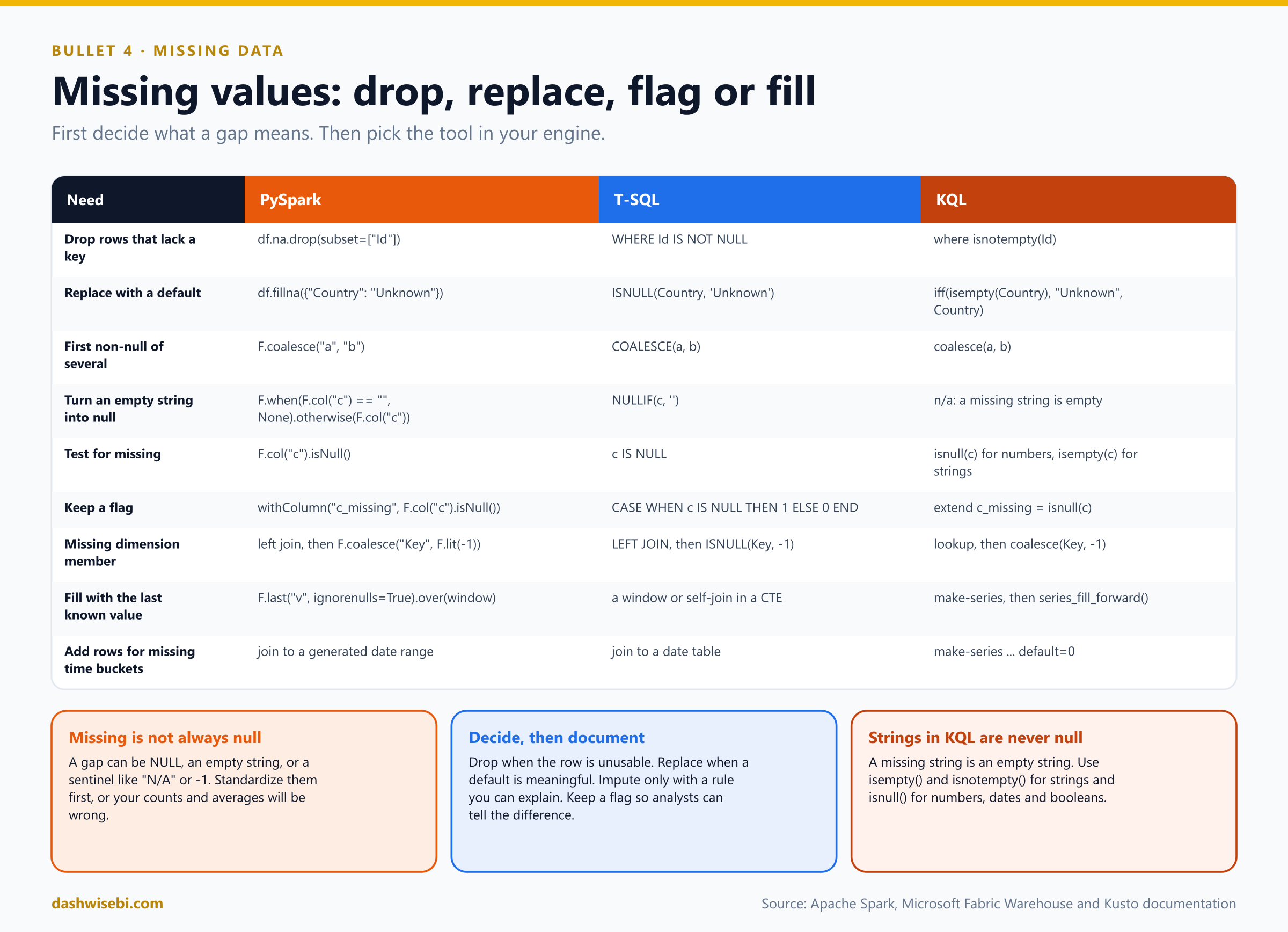
Some details matter:
fillnais type-aware. A string default fills only string columns and a number fills only numeric ones.df.fillna({"Country": "Unknown", "Qty": 0})sets each column's own default.- Strings in KQL are never null. A missing string is an empty string, so use
isempty()andisnotempty()for text. Useisnull()for numbers, dates and booleans. NULLIF(c, '')turns an empty string into null in T-SQL, which makesCOALESCEand aggregates behave.- Do not use 0 for a missing average input. Replacing nulls with 0 lowers the average. Leave them null, which the aggregate skips, or impute deliberately.
- Missing dimension member. Left join and set the key to the Unknown member (
-1), as in Episode 5. Never drop the fact row. - Fill forward. For sensor-like data, carry the last known value forward. In Spark use
last(..., ignorenulls=True)over a window. In KQL usemake-seriesandseries_fill_forward().make-seriesalso creates the rows for time buckets that have no data, with a default value.
from pyspark.sql import Window
w = (Window.partitionBy("DeviceId").orderBy("Ts")
.rowsBetween(Window.unboundedPreceding, Window.currentRow))
filled = readings.withColumn("Temp", F.last("Temp", ignorenulls=True).over(w))Readings
| make-series Temp = avg(Temp) default=real(null)
on Ts from datetime(2026-11-01) to datetime(2026-11-02) step 1h by DeviceId
| extend Temp = series_fill_forward(Temp)From the demo: profile, standardize and fill
The order is always profile, standardize placeholders, then decide. Counting only nulls hides most of the junk.
PySpark. First count the nulls in every column, then standardize the text:
display(orders_dedup.select([F.sum(F.col(c).isNull().cast("int")).alias(c)
for c in orders_dedup.columns]))Only one Country shows as null, but N/A, " india " and india are problems too.
PLACEHOLDERS = ["", "N/A", "NA", "NULL", "-", "UNKNOWN"]
orders_std = orders_dedup.withColumn(
"Country",
F.when(F.upper(F.trim("Country")).isin(PLACEHOLDERS), F.lit(None))
.when(F.length(F.trim("Country")) <= 3, F.upper(F.trim("Country"))) # codes: UK, USA
.otherwise(F.initcap(F.trim("Country"))) # names: India
)
display(orders_std.groupBy("Country").count().orderBy("Country"))- Placeholders become real nulls:
isin(PLACEHOLDERS)on the trimmed, upper-cased country catches"",N/A,NA,NULL,-andUNKNOWNin any case. - Short values (3 characters or fewer) are treated as codes and upper-cased (
UK,USA). Longer values are names and getinitcap(India). Now" india ",indiaandIndiaare one value.
Filling with 0 distorts averages. Compare the average quantity with the nulls ignored against the one after filling them with 0:
filled_zero = orders_std.fillna({"Country": "Unknown", "Qty": 0})
display(
orders_std.agg(F.avg("Qty").alias("AvgQty_nulls_ignored"))
.crossJoin(filled_zero.agg(F.avg("Qty").alias("AvgQty_after_fill_0")))
)The second average is lower, because the missing quantity now counts as a real zero. The demo's decision for silver is to fill Country with "Unknown", keep Qty as null, and add a flag so the gap stays visible:
orders_clean = (orders_std
.withColumn("QtyMissing", F.col("Qty").isNull())
.fillna({"Country": "Unknown"}))
display(orders_clean.orderBy("OrderID"))T-SQL. The profile counts nulls and placeholders, and trailing spaces:
SELECT SUM(CASE WHEN Qty IS NULL THEN 1 ELSE 0 END) AS QtyNull,
SUM(CASE WHEN Country IS NULL THEN 1 ELSE 0 END) AS CountryNull,
SUM(CASE WHEN UPPER(TRIM(Country)) IN ('', 'N/A', 'NA', 'NULL', '-', 'UNKNOWN')
THEN 1 ELSE 0 END) AS CountryPlaceholder,
SUM(CASE WHEN Country <> TRIM(Country) THEN 1 ELSE 0 END) AS CountryNeedsTrim
FROM ep7.OrdersTyped;Standardizing needs more code than in Spark, because T-SQL has no INITCAP:
SELECT Country AS CountryRaw,
CASE WHEN Country IS NULL
OR UPPER(TRIM(Country)) IN ('', 'N/A', 'NA', 'NULL', '-', 'UNKNOWN') THEN NULL
WHEN LEN(TRIM(Country)) <= 3 THEN UPPER(TRIM(Country)) -- UK, USA
ELSE UPPER(LEFT(TRIM(Country), 1)) + LOWER(SUBSTRING(TRIM(Country), 2, 100)) -- India
END AS CountryClean,
COUNT(*) AS Rows
FROM ep7.OrdersTyped
GROUP BY Country;The CASE expression makes placeholders NULL, upper-cases short codes, and builds the capitalized name by hand from UPPER(LEFT(...)) + LOWER(SUBSTRING(...)). The same average trap, in SQL:
SELECT AVG(CAST(Qty AS DECIMAL(10,4))) AS AvgQty_NullsIgnored,
AVG(CAST(ISNULL(Qty, 0) AS DECIMAL(10,4))) AS AvgQty_After_ISNULL_0
FROM (SELECT *, ROW_NUMBER() OVER (PARTITION BY OrderID ORDER BY ModifiedAt DESC) AS rn
FROM ep7.OrdersTyped) t
WHERE rn = 1;AVG ignores nulls, and ISNULL(Qty, 0) lowers the average. The ROW_NUMBER() subquery keeps only the latest version of each order first.
Fill forward has no one-word function in T-SQL, but there is a neat trick:
WITH prices AS
(
SELECT * FROM (VALUES ('P01', CAST('2026-11-01' AS DATE), CAST(25.0 AS DECIMAL(10,2))),
('P01', CAST('2026-11-02' AS DATE), CAST(NULL AS DECIMAL(10,2))),
('P01', CAST('2026-11-03' AS DATE), CAST(NULL AS DECIMAL(10,2))),
('P01', CAST('2026-11-04' AS DATE), CAST(26.0 AS DECIMAL(10,2))),
('P02', CAST('2026-11-01' AS DATE), CAST(120.0 AS DECIMAL(10,2))),
('P02', CAST('2026-11-02' AS DATE), CAST(NULL AS DECIMAL(10,2)))) v(ProductID, PriceDate, Price)
),
grouped AS
(
SELECT *, COUNT(Price) OVER (PARTITION BY ProductID ORDER BY PriceDate ROWS UNBOUNDED PRECEDING) AS grp
FROM prices
)
SELECT ProductID, PriceDate, Price,
MAX(Price) OVER (PARTITION BY ProductID, grp) AS PriceFilled
FROM grouped
ORDER BY ProductID, PriceDate;COUNT(Price) OVER (...) counts only non-null prices, so the number grows only on rows that have a price. Each null row therefore shares the group number of the last known price, and MAX(Price) OVER (PARTITION BY ProductID, grp) copies that price to every row of the group.
KQL. Strings are empty, never null, so the profile must use both tests:
OrdersLatest
| summarize QtyIsNull = countif(isnull(Qty)),
CountryIsNull = countif(isnull(Country)),
CountryEmpty = countif(isempty(Country)),
Rows = count(), // count() counts ROWS, not non-null values
RowsWithQty = countif(isnotnull(Qty))CountryIsNull is 0 even though one country is missing, because that value is an empty string. CountryEmpty finds it. Standardizing placeholders, and then the trap:
OrdersLatest
| extend c = trim(@"\s+", Country)
| extend CountryClean = case(toupper(c) in ("", "N/A", "NA", "NULL", "-", "UNKNOWN"), "Unknown",
strlen(c) <= 3, toupper(c),
strcat(toupper(substring(c, 0, 1)), tolower(substring(c, 1))))
| summarize Rows = count() by CountryRaw = Country, CountryCleanOrdersLatest
| where OrderID == 1008
| project OrderID, Country,
WithCoalesce = coalesce(Country, "Unknown"),
WithIff = iff(isempty(Country), "Unknown", Country)For order 1008, the country is an empty string. coalesce(Country, "Unknown") returns the empty string, not "Unknown", because an empty string is not null. iff(isempty(Country), "Unknown", Country) is the correct way for text. Averages behave as elsewhere:
OrdersLatest
| summarize AvgQty_NullsIgnored = avg(Qty),
AvgQty_Fill0 = avg(coalesce(Qty, int(0)))And the KQL fill forward, make-series to create the missing days and series_fill_forward() to carry the last value into them:
datatable(ProductID:string, PriceDate:datetime, Price:real)
[
"P01", datetime(2026-11-01), 25.0,
"P01", datetime(2026-11-04), 26.0,
"P02", datetime(2026-11-01), 120.0
]
| make-series Price = avg(Price) default = real(null)
on PriceDate from datetime(2026-11-01) to datetime(2026-11-05) step 1d
by ProductID
| extend PriceFilled = series_fill_forward(Price)
| mv-expand PriceDate to typeof(datetime), Price to typeof(real), PriceFilled to typeof(real)
| order by ProductID asc, PriceDate ascProduct P01 has prices on 1 and 4 November only. make-series creates a row for every day with a null where there is no price, series_fill_forward fills the nulls, and mv-expand turns the arrays back into rows.
Late-arriving data
Every record has two times: event time (when it happened) and arrival time (when it reached Fabric). Data is late when it arrives after the load that should have included it. Batch pipelines have this problem too, not just streams.
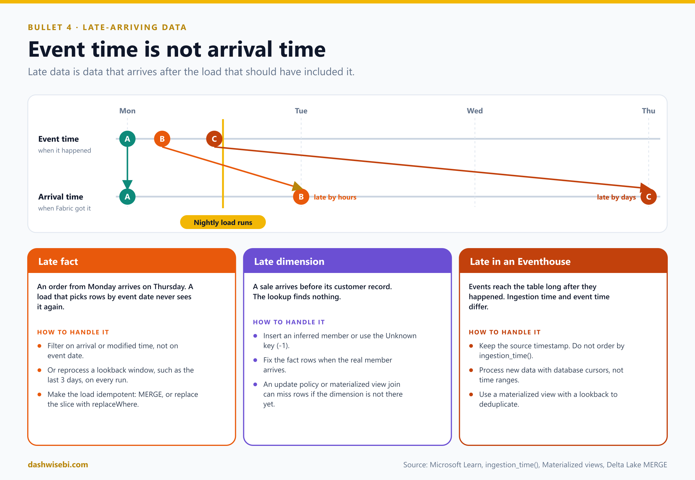
Late-arriving facts
An order from Monday shows up on Thursday. If your incremental load selects rows by event date (OrderDate = yesterday), it never sees that row. There are three fixes:
- Filter on arrival or modified time. A watermark on
ModifiedAtorIngestedAtcatches late rows, as in the watermark pipeline from Episode 5. - Reprocess a lookback window. Every run re-reads, say, the last three days from the source, and replaces or merges that window. Late rows inside the window are caught.
- Make the load idempotent. Use
MERGE, or replace the slice with Delta'sreplaceWhereoption so rerunning gives the same table:
window_start = "2026-11-01" # re-read the last N days on every run
fresh = spark.table("bronze_orders").where(f"OrderDate >= '{window_start}'")
(fresh.write.format("delta").mode("overwrite")
.option("replaceWhere", f"OrderDate >= '{window_start}'")
.saveAsTable("silver_orders"))Late facts also change aggregates you already published. Decide whether to restate history or to lock periods, and tell your users which.
Late-arriving dimensions
A sale arrives before the customer record. The lookup finds no match. Do not drop the row and do not leave a null key. Insert an inferred member (a placeholder dimension row with the business key and unknown attributes) or use the Unknown member (-1), then update the dimension and repair the fact rows when the real data arrives. For a type 2 dimension, a late change also means closing and opening versions with corrected dates and pointing the affected facts at the right version.
Late data in an Eventhouse
ingestion_time()returns approximately when a record was ingested, in UTC. It returns null if the IngestionTime policy was not enabled when the data was ingested, and null when used outside a table or materialized view. It is approximate, and it is measured at the end of ingestion, so you cannot use it to order records. Keep the timestamp from the source system for ordering.- To process each record exactly once, use database cursors, not a time range.
- A materialized view includes late rows in its aggregate. A deduplication view with a lookback only compares against recently ingested records, so a repeat that arrives after the window is not caught.
- Update policies and joins. Update policies and materialized views can use joins, but only if the matching data is available when they run. If the dimension row is ingested after the fact, the policy can miss it. Load dimensions first, or enrich later at query time with
lookup.
Orders
| extend IngestedAt = ingestion_time()
| where IngestedAt > ago(1h) // arrived in the last hour, even if the event is old
| summarize Arrived = count(), OldestEvent = min(Timestamp)Streaming engines handle lateness with watermarks: a threshold such as "accept events up to 10 minutes late". We cover them in the streaming episodes. For batch, lookback windows and idempotent loads do the same job.
From the demo: batch 2 arrives
Batch 2 lands on 2026-11-10: an update to 1002 (Delivered), a late fact 1010 (an October order), a new order 1015 from the not-yet-known customer C005, a repeat of 1013, and a new Channel column. Every engine handles the same five steps.
1. Schema drift. A new column arrives in the file. Let the table grow instead of failing:
orders_batch_02 = """OrderID,CustomerID,ProductID,OrderDate,Qty,UnitPrice,Country,Status,ModifiedAt,Channel
1002,C002,P02,2026-10-01,1,120.00,India,Delivered,2026-11-10 09:00:00,Web
1010,C001,P03,2026-10-03,2,15.50,India,Shipped,2026-11-10 09:05:00,Store
1015,C005,P01,2026-11-09,2,25.00,Germany,Shipped,2026-11-10 09:10:00,Web
1013,C002,P01,2026-11-02,6,25.00,India,Shipped,2026-11-02 10:00:00,Web
"""
write_text(f"{LANDING_FS}/orders/orders_batch_02.csv", orders_batch_02)
bronze_b2 = (spark.read.option("header", True)
.csv(f"{LANDING_SPARK}/orders/orders_batch_02.csv")
.withColumn("_source_file", F.col("_metadata.file_path"))
.withColumn("_ingested_at", F.current_timestamp()))
# Schema drift: append the new Channel column with mergeSchema (old rows get null)
(bronze_b2.write.mode("append").option("mergeSchema", True).saveAsTable(f"{P}bronze_orders"))
spark.table(f"{P}bronze_orders").printSchema()
display(spark.table(f"{P}bronze_orders").groupBy("_source_file").count())In Spark, option("mergeSchema", True) adds the new column to the Delta table, and old rows get null in it. In T-SQL you add a nullable column and then insert the new rows:
ALTER TABLE ep7.StagingOrders ADD Channel VARCHAR(20) NULL;INSERT INTO ep7.StagingOrders
(OrderID, CustomerID, ProductID, OrderDate, Qty, UnitPrice, Country, Status, ModifiedAt, Channel, SourceFile, LoadedAt)
VALUES ('1002','C002','P02','2026-10-01','1','120.00','India' ,'Delivered','2026-11-10 09:00:00','Web' ,'orders_batch_02.csv',SYSUTCDATETIME()),
('1010','C001','P03','2026-10-03','2','15.50' ,'India' ,'Shipped' ,'2026-11-10 09:05:00','Store','orders_batch_02.csv',SYSUTCDATETIME()),
('1015','C005','P01','2026-11-09','2','25.00' ,'Germany','Shipped' ,'2026-11-10 09:10:00','Web' ,'orders_batch_02.csv',SYSUTCDATETIME()),
('1013','C002','P01','2026-11-02','6','25.00' ,'India' ,'Shipped' ,'2026-11-02 10:00:00','Web' ,'orders_batch_02.csv',SYSUTCDATETIME());In KQL, .alter-merge adds the column, and the materialized views follow because of autoUpdateSchema=true. The batch is tagged and protected with ingestIfNotExists:
.alter-merge table Orders (Channel:string)
.ingest inline into table Orders with (format="csv", tags='["ingest-by:orders_batch_02"]', ingestIfNotExists='["orders_batch_02"]') <|
1002,C002,P02,2026-10-01,1,120.00,India,Delivered,2026-11-10 09:00:00,Web
1010,C001,P03,2026-10-03,2,15.50,India,Shipped,2026-11-10 09:05:00,Store
1015,C005,P01,2026-11-09,2,25.00,Germany,Shipped,2026-11-10 09:10:00,Web
1013,C002,P01,2026-11-02,6,25.00,India,Shipped,2026-11-02 10:00:00,Web2. Event date versus watermark. The naive load takes rows with an OrderDate later than the last loaded date. The correct load takes rows whose ModifiedAt is later than the watermark:
silver_now = spark.table(f"{P}silver_orders")
last_event_date = silver_now.agg(F.max("OrderDate")).first()[0]
watermark = silver_now.agg(F.max("ModifiedAt")).first()[0]
print("Last OrderDate in silver:", last_event_date, "| Watermark (max ModifiedAt):", watermark)
bronze_typed = to_silver(spark.table(f"{P}bronze_orders"))
naive = bronze_typed.where(F.col("OrderDate") > F.lit(last_event_date))
incremental = bronze_typed.where(F.col("ModifiedAt") > F.lit(watermark))
print("Naive event-date load picks up:", [r.OrderID for r in naive.collect()])
print("Watermark load picks up: ", sorted(r.OrderID for r in incremental.collect()))The naive load finds only 1015, so it misses the late order 1010 and the update to 1002. The watermark load finds 1002, 1010 and 1015, and correctly skips the repeat 1013, whose ModifiedAt is not newer. The same comparison in T-SQL and KQL:
DECLARE @LastEventDate DATE = (SELECT MAX(OrderDate) FROM ep7.SilverOrders);
DECLARE @Watermark DATETIME2(6) = (SELECT MAX(ModifiedAt) FROM ep7.SilverOrders);
SELECT 'Naive: OrderDate > last loaded date' AS Approach, OrderID, OrderDate, ModifiedAt, Status
FROM ep7.vw_SilverCandidates WHERE OrderDate > @LastEventDate -- only 1015: misses 1002 + 1010
UNION ALL
SELECT 'Watermark: ModifiedAt > max(ModifiedAt)', OrderID, OrderDate, ModifiedAt, Status
FROM ep7.vw_SilverCandidates WHERE ModifiedAt > @Watermark -- 1002, 1010, 1015
ORDER BY Approach, OrderID;let LastEventDate = datetime(2026-11-05);
let Watermark = datetime(2026-11-05 11:00:00);
union
(OrdersLatest | where OrderDate > LastEventDate | extend Approach = "Naive: OrderDate > last loaded date"),
(OrdersLatest | where ModifiedAt > Watermark | extend Approach = "Watermark: ModifiedAt > max(ModifiedAt)")
| project Approach, OrderID, OrderDate, ModifiedAt, Status
| order by Approach asc, OrderID asc3. Load with a lookback window, then run it again. A lookback re-reads everything modified in the last N days. The overlap is deliberate, and the guard makes it harmless:
LOOKBACK_DAYS = 14
lookback = bronze_typed.where(F.col("ModifiedAt") >= F.lit(watermark) - F.expr(f"INTERVAL {LOOKBACK_DAYS} DAYS"))
print("Lookback picks up:", sorted(r.OrderID for r in lookback.collect()))
upsert_silver(lookback)
display(last_merge_metrics(f"{P}silver_orders"))
display(spark.table(f"{P}silver_orders").where("OrderID IN (1002, 1010, 1013, 1015)").orderBy("OrderID"))# Run batch 2 again: nothing should change
before = fingerprint(f"{P}silver_orders")
upsert_silver(lookback)
print("Idempotent on rerun:", before == fingerprint(f"{P}silver_orders"))The rerun check prints True when the table is unchanged. In T-SQL, call the procedure from earlier twice, and compare with the snapshot:
EXEC ep7.usp_LoadSilver @LookbackDays = 14;DROP TABLE IF EXISTS ep7.SilverSnapshot;
CREATE TABLE ep7.SilverSnapshot AS SELECT * FROM ep7.SilverOrders;
GO
EXEC ep7.usp_LoadSilver @LookbackDays = 14;
GO
SELECT  (SELECT COUNT(*) FROM (SELECT * FROM ep7.SilverOrders   EXCEPT SELECT * FROM ep7.SilverSnapshot) a) AS RowsAdded,
(SELECT COUNT(*) FROM (SELECT * FROM ep7.SilverSnapshot EXCEPT SELECT * FROM ep7.SilverOrders) b) AS RowsLost;In the Eventhouse, the materialized views take care of this on their own. After batch 2, OrdersLatest shows 1002 as Delivered and includes the late 1010, and OrdersDedup counts the repeated 1013 once:
OrdersLatest
| where OrderID in (1002, 1010, 1013, 1015)
| project OrderID, OrderDate, Status, ModifiedAt, Channel
| order by OrderID asc

OrdersDedup
| where OrderID == 1013
| count
4. Arrival time in an Eventhouse. ingestion_time() returns the (approximate) arrival time. Every row of a batch shares almost the same value, so it is good for finding "what is new" but not for ordering events:
Orders
| extend IngestedAt = ingestion_time()
| summarize Rows = count(), DistinctIngestTimes = dcount(IngestedAt), FirstIngest = min(IngestedAt), LastIngest = max(IngestedAt)
For exactly-once processing downstream, use a database cursor: save cursor_current() after each run and, next time, read only Orders | where cursor_after('<saved cursor>').
print CurrentCursor = cursor_current()5. The late dimension. Customer C005 finally arrives. In the lakehouse and the Warehouse, gold is rebuilt from silver, so adding the row and rebuilding repairs orders 1009 and 1015. Nothing needs backfilling, because the fact rows were never dropped:
print("Before: rows on Unknown customer")
display(spark.table(f"{P}gold_sales_wide").where("CustomerKey = -1").select("OrderID", "SourceCustomerID", "CustomerKey"))

spark.createDataFrame([(5, "C005", "Eagle GmbH", "Corporate", "Berlin")],
                      spark.table(f"{P}src_customer").schema) \
     .write.mode("append").saveAsTable(f"{P}src_customer")

build_dim_customer()
build_gold_sales_wide()

print("After: only the customer that never existed (C999) is still Unknown")
display(spark.table(f"{P}gold_sales_wide").where("CustomerKey = -1 OR SourceCustomerID = 'C005'")
                                          .select("OrderID", "SourceCustomerID", "CustomerKey", "CustomerName"))
INSERT INTO ep7.SrcCustomer VALUES (5, 'C005', 'Eagle GmbH', 'Corporate', 'Berlin');EXEC ep7.usp_BuildGold;SELECT OrderID, SourceCustomerID, CustomerKey, CustomerName
FROM ep7.FactSalesWide
WHERE CustomerKey = -1 OR SourceCustomerID = 'C005'
ORDER BY OrderID; -- only C999 stays on -1After the rebuild, only customer C999, who never existed, stays on the Unknown member.
The Eventhouse behaves differently, and this is a classic exam question. The update policy enriched 1009 and 1015 before C005 existed, so their customer name is empty:
OrdersEnriched
| where CustomerID == "C005"
| project OrderID, CustomerID, CustomerName
.append Customers <|
datatable(CustomerID:string, CustomerName:string, Segment:string, City:string)
[ "C005", "Eagle GmbH", "Corporate", "Berlin" ]After C005 is appended, query the enriched table again. The names are still empty, because an update policy runs once, at ingestion, and never reruns. The query-time function is correct immediately:
SalesWide
| where CustomerID == "C005"
| project OrderID, CustomerID, CustomerName
To repair the ingestion-time table, backfill: rerun the enrichment over the whole table. Outside the policy, EnrichOrders() reads all of Orders, not just one batch:
.set-or-replace OrdersEnriched <|
EnrichOrders()
So there are three answers to "enrichment is null for a late dimension": load dimensions first, enrich at query time, or backfill once the dimension arrives.
6. Restate only the affected dates. Instead of overwriting the whole daily table, recompute only the date range that this batch touched. In Delta this is replaceWhere:
affected = lookback.agg(F.min("OrderDate").alias("lo"), F.max("OrderDate").alias("hi")).first()
predicate = f"OrderDate >= '{affected.lo}' AND OrderDate <= '{affected.hi}'"
print("Replacing slice:", predicate)

restated = (spark.table(f"{P}gold_sales_wide")
                 .where("Status <> 'Cancelled'")
                 .where(predicate)
                 .groupBy("OrderDate").agg(F.sum("LineAmount").alias("Revenue")))

(restated.write.mode("overwrite")
         .option("replaceWhere", predicate)
         .saveAsTable(f"{P}gold_daily_sales"))

display(spark.table(f"{P}gold_daily_sales").orderBy("OrderDate"))- The predicate is built from the smallest and largest
OrderDatein the batch.replaceWherereplaces only the rows that match the predicate and fails if the new data falls outside it. - Running it again gives the same result, so it is idempotent, and it is much cheaper than rewriting a big table.
The Warehouse has no replaceWhere, so it restates the slice with a transaction: delete the range and insert it again. If anything fails, the transaction rolls back, and the table never shows a half-restated state:
DECLARE @lo DATE = (SELECT MIN(TRY_CAST(OrderDate AS DATE)) FROM ep7.StagingOrders WHERE SourceFile = 'orders_batch_02.csv');
DECLARE @hi DATE = (SELECT MAX(TRY_CAST(OrderDate AS DATE)) FROM ep7.StagingOrders WHERE SourceFile = 'orders_batch_02.csv');

BEGIN TRANSACTION;
    DELETE FROM ep7.DailyRevenue WHERE OrderDate BETWEEN @lo AND @hi;

    INSERT INTO ep7.DailyRevenue (OrderDate, Revenue)
    SELECT OrderDate, SUM(LineAmount)
    FROM ep7.FactSalesWide
    WHERE Status <> 'Cancelled' AND OrderDate BETWEEN @lo AND @hi
    GROUP BY OrderDate;
COMMIT TRANSACTION;

SELECT @lo AS RestatedFrom, @hi AS RestatedTo;
SELECT * FROM ep7.DailyRevenue ORDER BY OrderDate;
Choosing the right pattern
Match the symptom to the fix. The first yes is your answer.
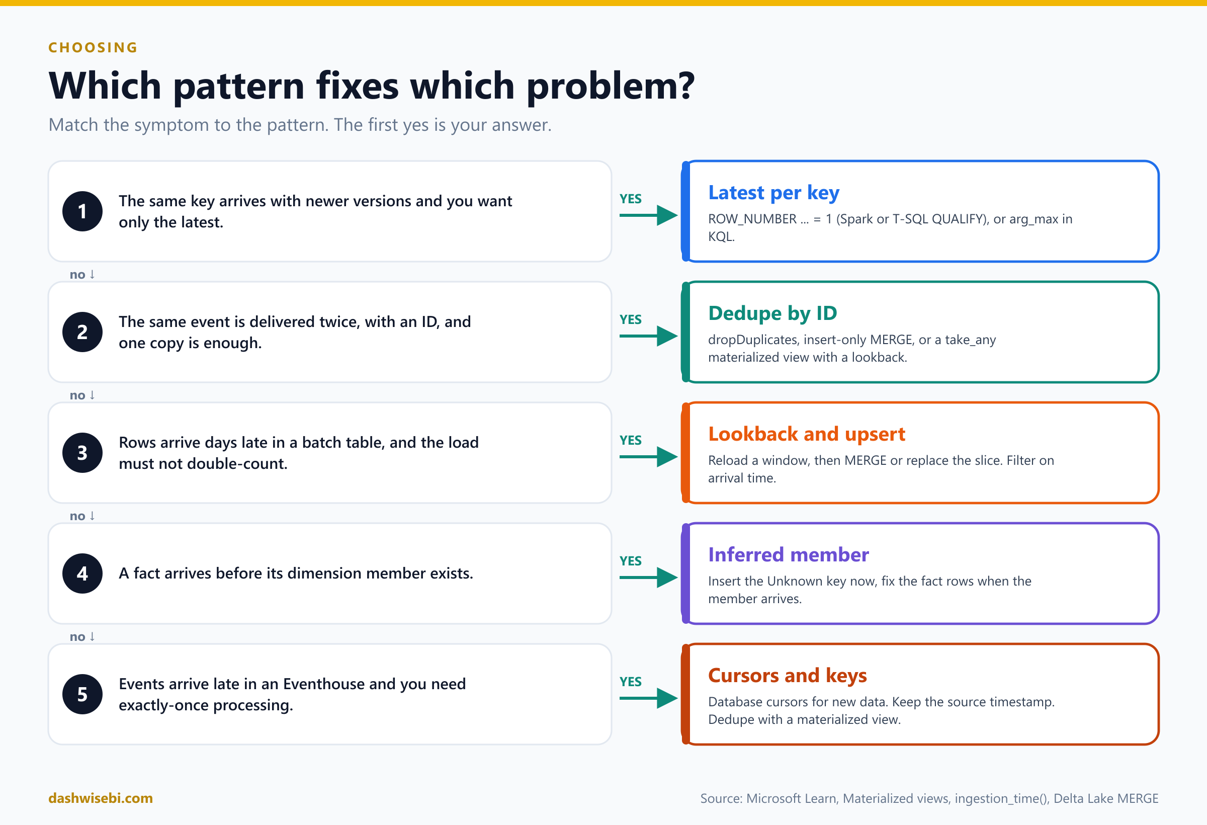
When an exam question describes a need, find it on the left and pick the answer on the right.
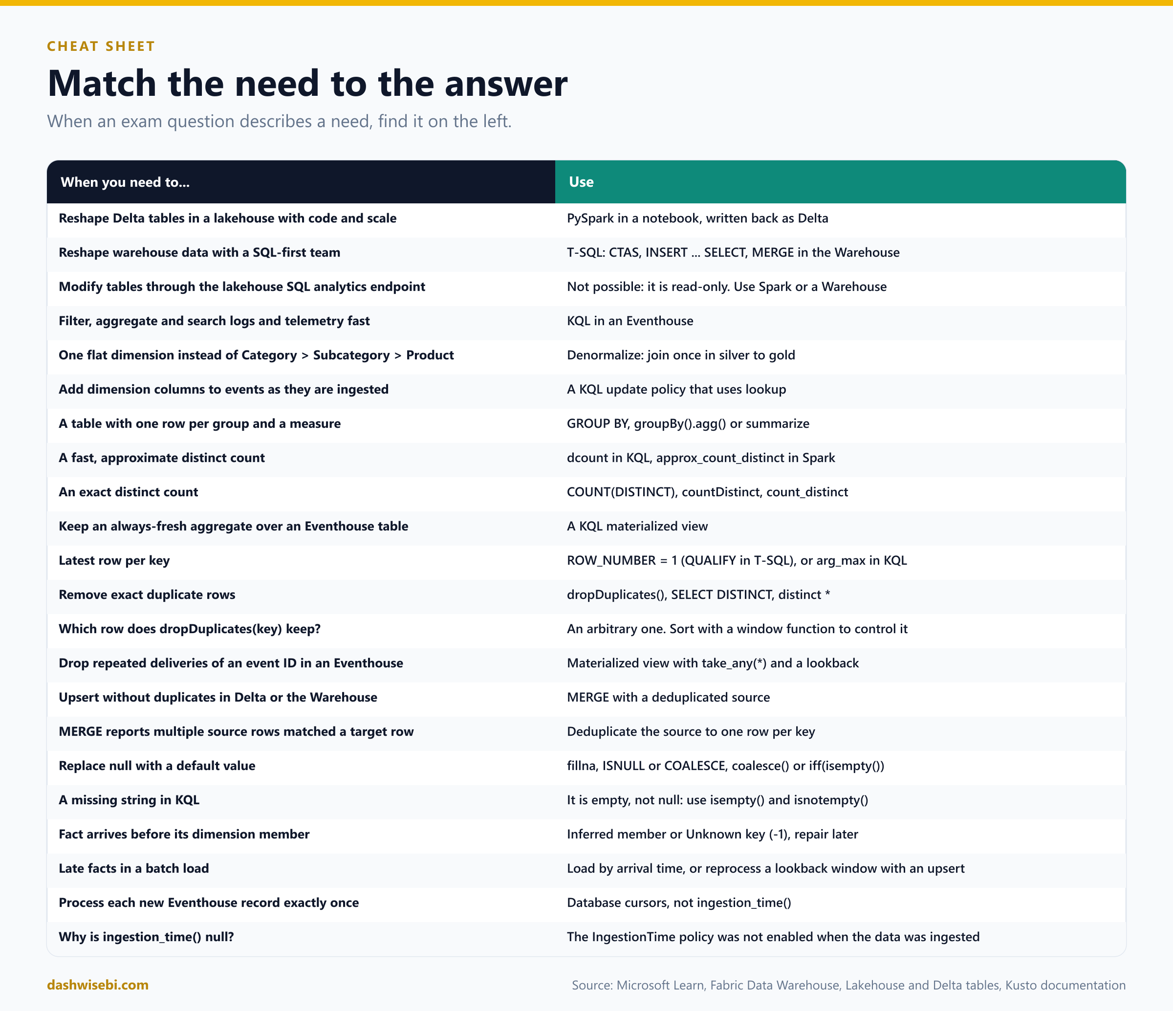
Common mix-ups
- "You can INSERT or UPDATE through the lakehouse SQL analytics endpoint." It is read-only. Write with Spark, a pipeline or a dataflow, or use the Warehouse for T-SQL writes.
- "The Warehouse supports triggers, recursive queries and materialized views." It does not. KQL has materialized views, and the Warehouse does not.
- "A primary key stops duplicates in the Warehouse." Keys are accepted only as
NOT ENFORCED. Your ETL must check them. - "PySpark runs each line as you type it." Transformations are lazy and run when an action such as
writeorcountis called. - "
dropDuplicates(key)keeps the newest row." It keeps an arbitrary one. Use a window function when the newest must win. - "
distinct()anddropDuplicates(subset)are the same."distinct()compares every column. - "
MERGEquietly picks one of several matching source rows." It fails or is ambiguous. Deduplicate the source to one row per key. - "The default KQL join is an inner join." It is
innerunique, which removes duplicate left keys first. - "
lookupworks with a big right-hand table." The right side is broadcast and should be small. A few tens of MB is the limit. - "A missing string in KQL is null." It is empty. Use
isempty(). - "KQL
count()skips nulls." It counts rows. Usecountif(isnotnull(x)). - "
dcount()is exact." It is approximate. Usecount_distinct()for exact. - "An aggregate over an empty table with no group-by returns no rows." It returns one row.
- "An update policy can aggregate across batches." It sees one ingestion batch. Use a materialized view.
- "Materialized views run during ingestion." They materialize in the background, but queries still see fresh data because the view adds the unprocessed records at query time.
- "A left join never changes the number of fact rows." It can multiply them if the dimension key is not unique.
- "Replace missing numbers with 0 for averages." That drags the average down. Leave nulls or impute with a rule.
- "
fillna(0)fills text columns too." A number fills only numeric columns. - "A load by event date catches late rows." It never revisits old dates. Load by arrival time or reprocess a lookback window.
- "Late data is only a streaming problem." Batch loads have it too.
- "Drop a fact row when its dimension is missing." Use the Unknown member and repair it later.
- "
ingestion_time()can order records." It cannot. It is approximate, and it is null if the policy was off at ingestion. - "An empty string cast to INT in T-SQL gives null."
TRY_CAST('' AS INT)returns 0, and an empty string cast to a date returns 1900-01-01. Wrap the value withNULLIF(TRIM(x), '')first. - "
coalesce(Country, "Unknown")fixes a missing country in KQL." A missing string is empty, not null, socoalescedoes nothing. Useiff(isempty(Country), "Unknown", Country). - "Loading the same batch twice is harmless in an Eventhouse." It doubles the rows. Use an
ingest-bytag withingestIfNotExists, or a deduplication view. - "A primary key in the Warehouse rejects a duplicate." The demo inserts two rows with the same key without an error, because the key is
NOT ENFORCED. - "Adding the late customer repairs the Eventhouse enrichment automatically." An update policy runs once, at ingestion. Backfill the table, or enrich at query time.
- "
explode,CROSS APPLYandmv-expandkeep orders with no items." They drop them. Useexplode_outer,OUTER APPLYor turn the empty array into[null]first. - "
unionin PySpark matches columns by name." It matches by position. UseunionByName.
Try these scenarios
Ten exam-style questions. Cover the answers and test yourself.
1. The slow product hierarchy
Every report joins Sales to Product, Subcategory and Category. The model is slow and report authors are confused. What do you change?
Answer: Denormalize. In the silver to gold step, join the three tables into one flat DimProduct with Product, Subcategory and Category (a CTAS in T-SQL, or joins in a notebook), and point the fact table at it.
2. The join that lost rows
A KQL query joins Events to Devices on DeviceId, and the result has fewer rows than Events. Why?
Answer: The default join kind is innerunique, which removes duplicate keys from the left table first, and it drops unmatched rows. Use kind=leftouter, or the lookup operator for a small dimension.
3. Writing from the SQL endpoint
A developer runs an INSERT against a lakehouse table through its SQL analytics endpoint and gets an error. What are the options?
Answer: The endpoint is read-only. Write the data with Spark (a notebook), a pipeline or a dataflow, or load it into a Warehouse, where T-SQL writes are supported.
4. The wrong order wins
A notebook uses dropDuplicates(["OrderId"]) on a bronze table that holds several versions of each order. Sometimes an old version survives. How do you fix it?
Answer: dropDuplicates keeps an arbitrary row. Use a window function: row_number() over partitionBy("OrderId") ordered by ModifiedAt descending, and keep row 1.
5. The failing merge
A Delta MERGE into silver_orders fails because several source rows match the same target row. What is the cause and the fix?
Answer: The source has duplicate keys. Deduplicate the source to one row per OrderId (latest by ModifiedAt) before the merge, and keep a s.ModifiedAt > t.ModifiedAt condition so a late older row never wins.
6. Events delivered twice
An eventstream delivers each event at least once. Analysts query an Eventhouse table and see duplicates, but only for repeats that arrive within a few hours. What is a low-effort fix?
Answer: A materialized view that groups by EventId with take_any(*) and a lookback of a few hours. Query the view instead of the raw table.
7. Orders that show up days late
A nightly load copies yesterday's rows by OrderDate. Finance reports that some orders are missing, and they appear in the source days later. What do you change?
Answer: Stop selecting by event date. Use a watermark on the modified or arrival time, or reprocess a lookback window (for example the last 3 days) on every run, and write it with MERGE or replaceWhere so the load is idempotent.
8. The enrichment that returns nulls
An update policy enriches telemetry with device details using lookup. For new devices the enriched columns are empty, even after the device record is loaded a minute later. Why?
Answer: The update policy ran at ingestion, when the device row did not exist yet, and it does not rerun. Load the dimension before the facts, or enrich at query time with lookup, or backfill the affected rows once the dimension arrives.
9. The zero that was never ordered
A Warehouse load casts an empty Qty column with TRY_CAST(Qty AS INT). An analyst notices orders with a quantity of 0, and the average quantity is too low. What happened, and what is the fix?
Answer: In T-SQL, casting an empty string gives 0, not null. Use TRY_CAST(NULLIF(TRIM(Qty), '') AS INT), so an empty value becomes NULL, which AVG then skips.
10. The retry that doubled the table
A pipeline ingests a file into an Eventhouse table. The activity fails after the load, the pipeline retries, and now every row exists twice. How do you stop the retry from duplicating data?
Answer: Tag the ingestion with an ingest-by: tag and set ingestIfNotExists to the same value. When an extent with that tag already exists, the retry is skipped. A take_any(*) materialized view with a lookback is the second line of defense for repeats the tag does not catch.
Where to go next
- Run the three demo files in this order: the notebook, the Warehouse script, then the Eventhouse script. After each batch, compare the numbers: 13 orders in silver and in
OrdersLatest, and the same rows on the Unknown member. When Spark, T-SQL and KQL agree, you have understood the pattern. - In a trial workspace, load a small orders file into a lakehouse with a notebook. Add duplicate rows, rows with missing values and an older version of an order. Clean it with
row_number,fillnaand aMERGE, and run the load twice to prove it is idempotent. - Rebuild the same clean-up in a Warehouse with CTAS,
QUALIFYandMERGE. - In an Eventhouse, ingest the same data twice and create a
take_anymaterialized view with a lookback. Compare the raw table and the view. Then usemake-seriesto fill a gap in a time series. - Flatten a JSON file with
explodeand withmv-expand, and compare the results. - Read the sources behind this post: DP-700 study guide, Lakehouse and Delta tables, T-SQL surface area in Fabric Data Warehouse, summarize operator, join operator, lookup operator, arg_max() aggregation function, ingestion_time(), Materialized views, Materialized views use cases, Update policy overview, Delta Lake: update and merge and PySpark DataFrame.dropDuplicates.
Keep reading
DP-700 Episode 11: Streaming II, Spark & KQL
DP-700 study guide told as a story: run Spark Structured Streaming in production, process data with KQL, and write tumbling, hopping, sliding and session windows.
DP-700 Episode 9: Resolving Errors II & Optimization I
DP-700 study guide: fix Eventstream, T-SQL and OneLake shortcut errors, then tune Lakehouse tables and pipeline Copy activities in Microsoft Fabric.