DP-700 Episode 11: Streaming II, Spark & KQL

PowerBI consultant ·
Saturday, 6:50 in the morning. The Pune Cyclothon starts at eight, and by now your phone has the bike-share dashboard open. Pings are arriving at twice the usual rate.
Karan, ops lead: Meera, you have the stream into Fabric from last time. Today it has to do real work. Four people are waiting.
You are Meera, the data engineer at RideWise, the (fictional) bike-share from Episode 10. Last time you chose the engine and built the Eventstream. This time you compute on the stream, and the three topics of this episode are the three tools you use:
- Process data by using Spark structured streaming
- Process data by using KQL
- Create windowing functions
Like the last few episodes, this post is a working day and not a reference list. Each chapter follows the same rhythm:
- The problem. Someone brings you a request.
- Pause and decide. Try the choice yourself first. The answer is behind a click.
- Why. The facts behind it, with diagrams and code.
- Exam lens. What the DP-700 tends to ask, and the traps.
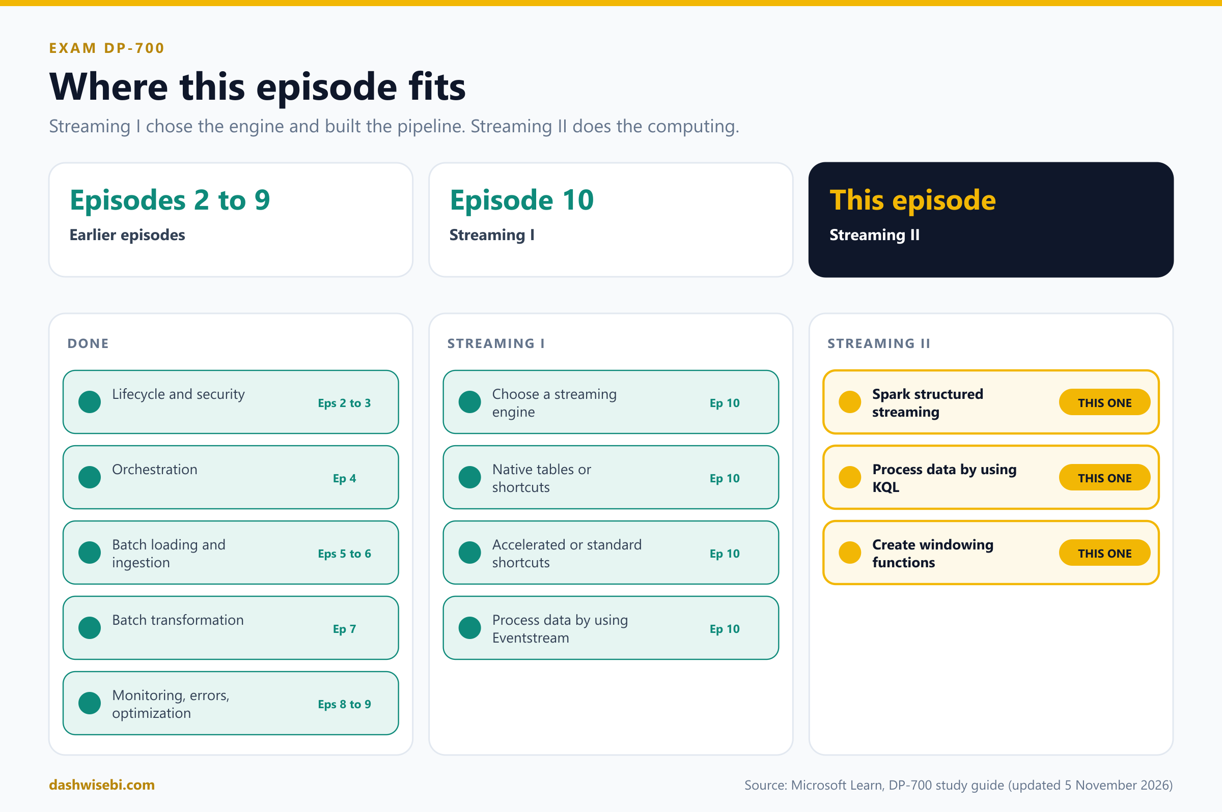
A note on wording. The study guide Microsoft updated on 5 November 2026 puts these topics in the group Ingest and transform streaming data. I follow Microsoft Learn, the Apache Spark guide and the Kusto reference, and I have not run every snippet on a live tenant. Where a feature is in preview, or where Learn says little, I say so. Before an exam, check the live documentation.
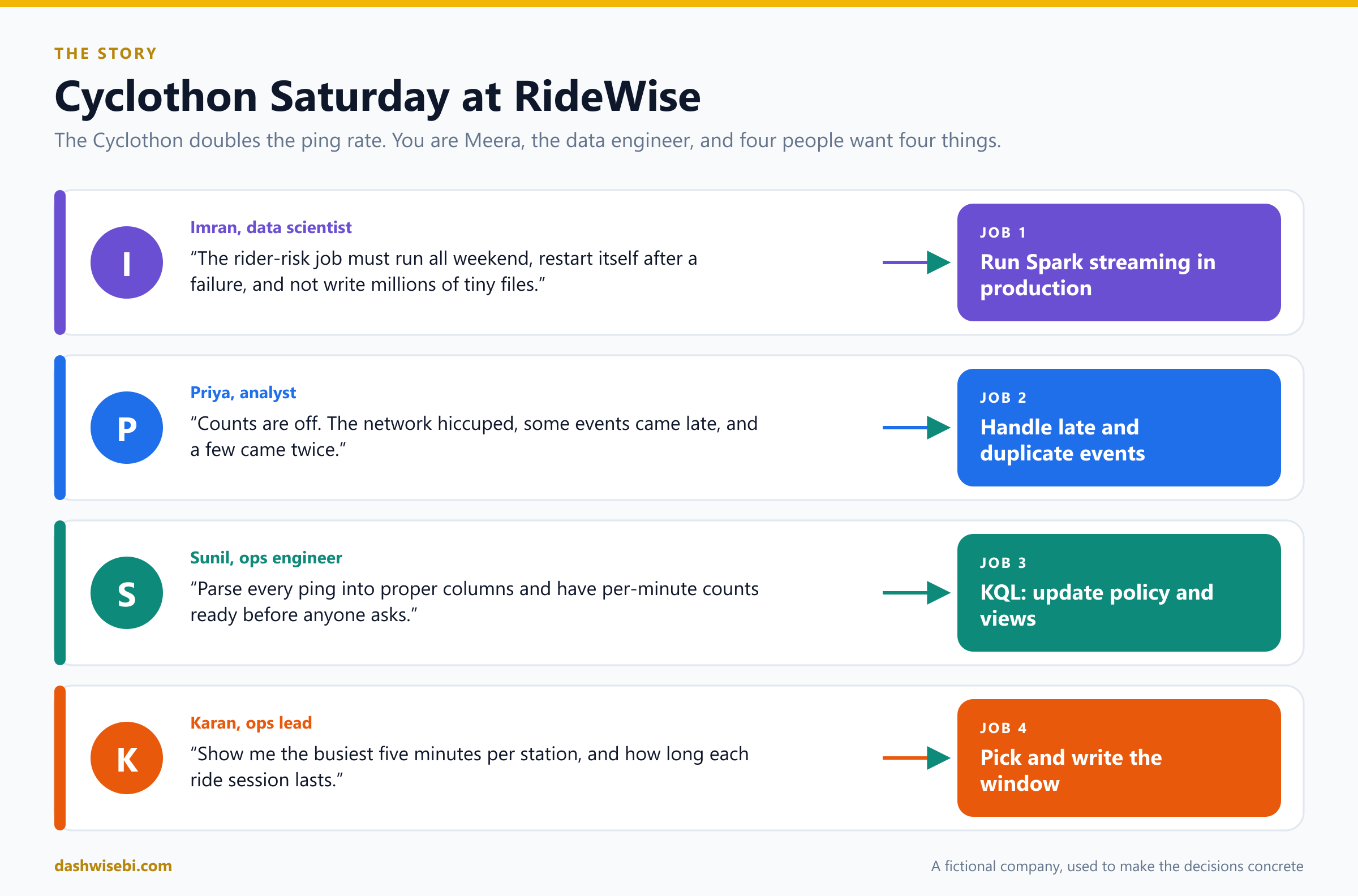
Chapter 1. Imran: the rider-risk job must survive the weekend
Imran arrives with a laptop and a tired face. “Last time my streaming notebook died at 3 a.m. and nobody noticed until noon. Today there are twice as many events, and I need it running until Monday.”
Imran's logic is custom Python, so it stays in Spark Structured Streaming, the engine you chose in Episode 10. The question now is how to run it in production. Try the decisions yourself.
Pause and decide. The job is developed in a notebook. For a job that must run continuously and restart itself, what do you run it as?
A Spark job definition. Notebooks are great for developing and testing streaming logic, but production jobs that need to run continuously belong in a job definition. It is non-interactive and code-oriented, and it offers a retry policy that restarts the job when hardware fails or infrastructure is patched.
Pause and decide. You turn the retry policy on. Where, and what do you set? Is there a catch?
Open the job's Settings, then the Optimization tab, and turn Retry Policy on. Set the maximum number of retry attempts (or allow unlimited attempts) and the time between attempts. The catch is a lifetime limit of 90 days. After that the policy stops working and the job is terminated. You restart it manually, which enables the policy again.
Pause and decide. The streaming job writes a Delta table, and the table is filling with thousands of tiny files. Name three levers.
(1) A trigger interval, such as trigger(processingTime="1 minute"), so Spark collects events and writes fewer, bigger files. (2) Optimized Write, enabled with spark.databricks.delta.optimizeWrite.enabled, which merges or splits partitions before writing, so you can drop manual repartition() and coalesce() calls. (3) Partitioning: partitionBy() on disk, and repartition() or coalesce() in memory.
Pause and decide. A partner drops a file into a folder every hour. Finance wants each file processed once, even after a restart, on a schedule. Which trigger?
trigger(availableNow=True). The query processes everything available, commits its progress to the checkpoint, and stops. A scheduler runs it again later, and the checkpoint remembers what is done. This is the same pattern from Episode 10.
Why: the anatomy of a streaming query
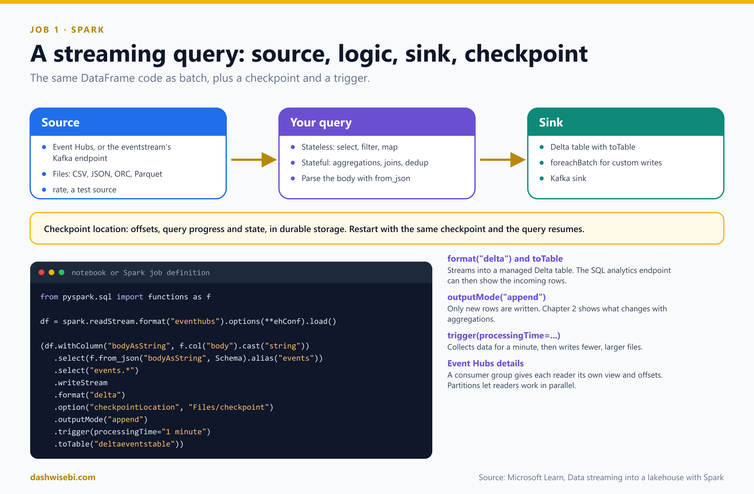
The Microsoft documentation shows the whole pattern in one chain. It reads from Event Hubs, parses the JSON in the message body, and writes to a managed Delta table:
import pyspark.sql.functions as f
from pyspark.sql.types import *

df = (
    spark.readStream
    .format("eventhubs")
    .options(**ehConf)
    .load()
)

Schema = StructType([
    StructField("bike_id", StringType(), False),
    StructField("station_id", StringType(), False),
    StructField("event_time", TimestampType(), True),
    StructField("battery", DoubleType(), True),
])

(df
    .withColumn("bodyAsString", f.col("body").cast("string"))
    .select(f.from_json("bodyAsString", Schema).alias("events"))
    .select("events.*")
    .writeStream
    .format("delta")
    .option("checkpointLocation", "Files/checkpoint")
    .outputMode("append")
    .trigger(processingTime="1 minute")
.toTable("pings_clean"))- Sources include built-in file sources (CSV, JSON, ORC, Parquet), Kafka and Azure Event Hubs. An eventstream exposes a Kafka-compatible endpoint, as you saw in Episode 10.
- Event Hubs consumer groups give each reading application its own view of the stream, at its own pace and with its own offsets. Partitions let readers work in parallel. Too many partitions for a low rate leaves readers idle, and high-throughput scenarios commonly use 32 or more.
format("delta")andtoTablestream straight into a managed Delta table with ACID guarantees. The SQL analytics endpoint of the lakehouse can then show the incoming rows.- The checkpoint keeps offsets, progress and state. One checkpoint per query, in durable storage.
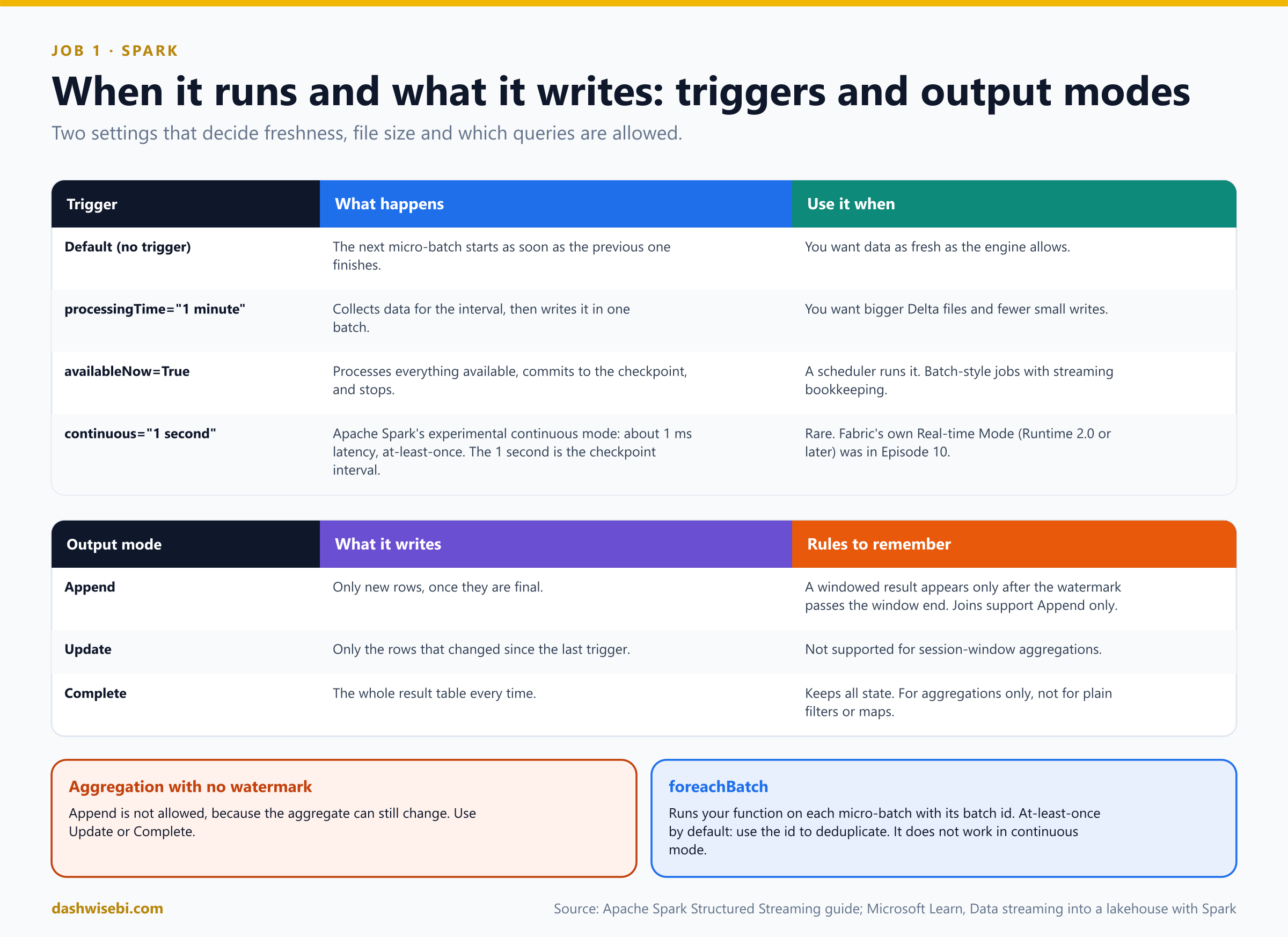
Triggers and output modes
- Default. The next micro-batch starts as soon as the previous one finishes.
processingTimebatches on an interval.availableNowprocesses what is there and stops.- Continuous is Apache Spark's experimental mode, with about 1 ms latency and at-least-once delivery. It is separate from Fabric's Real-time Mode (Runtime 2.0 or later) from Episode 10.
- Append writes only new rows once they are final. Update writes the rows that changed. Complete rewrites the whole result and keeps all state, so it is for aggregations.
- An aggregation with no watermark cannot use Append, because the aggregate can still change.
Pause and decide. Imran's job aggregates returns per station with no watermark. Which output modes can it use?
Update or Complete. Without a watermark, Spark cannot know when an aggregate is final, so Append is not allowed. Complete keeps all state, which grows. Add a watermark (Chapter 2) and Append becomes possible.
Pause and decide. Imran also wants each micro-batch written to two tables. Which sink option, and what does it guarantee?
foreachBatch. Your function receives each micro-batch as a DataFrame with a batch id. It gives at-least-once guarantees by default, so use the batch id to deduplicate if you need exactly-once behavior. If you write to several places, persist() the batch first so Spark does not recompute it. It does not work in continuous mode.
def write_two(batch_df, batch_id):
    batch_df.persist()
    batch_df.write.mode("append").saveAsTable("pings_clean")
    batch_df.write.mode("append").saveAsTable("pings_audit")
    batch_df.unpersist()

(events.writeStream
    .foreachBatch(write_two)
    .option("checkpointLocation", "Files/checkpoint_two")
    .start())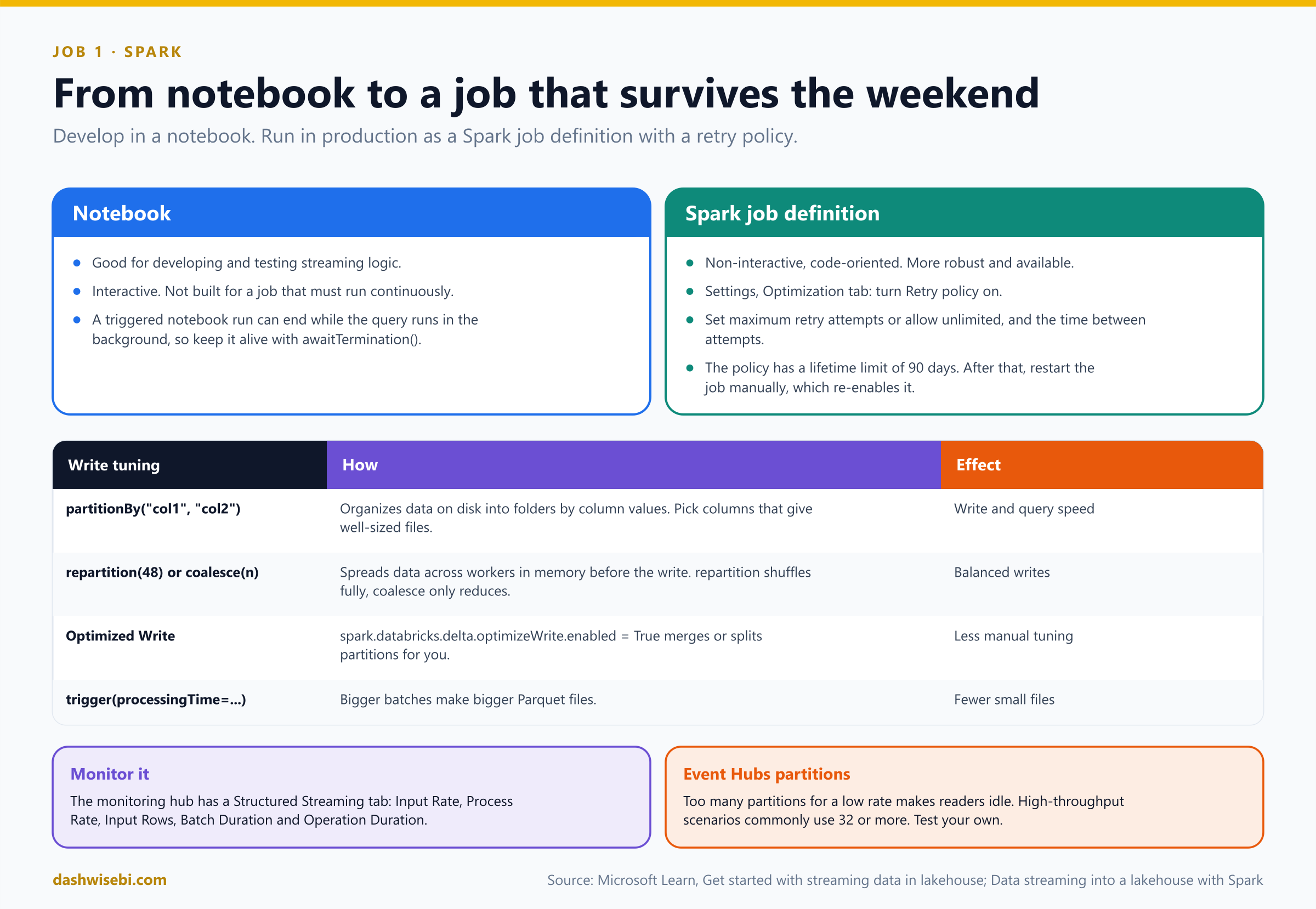
Running it in production
- Notebook to develop, job definition to run. A triggered notebook run can reach a terminal state while the query runs in the background, so keep it alive with
awaitTermination(). - Retry policy: maximum attempts or unlimited, interval between attempts, and a 90-day lifetime.
- Monitor in the monitoring hub. Its Structured Streaming tab shows Input Rate, Process Rate, Input Rows, Batch Duration and Operation Duration. A process rate lower than the input rate means the job is falling behind.
By 7:30 the job is a Spark job definition with a retry policy and a one-minute trigger. Imran reads the monitoring hub, nods, and goes to find coffee. You turn to the next sticky note.
Exam lens
- Production streaming in Spark: Spark job definition, retry policy (90-day limit), checkpoint per query.
- Small files: processingTime trigger, Optimized Write, partitioning.
- availableNow for scheduled runs. Append needs a watermark for aggregations. foreachBatch is at-least-once.
Chapter 2. Priya: the counts are wrong
Priya turns her laptop towards you. The station-minute counts do not match the trip totals. “The network at the stadium hiccuped. Some pings arrived ten minutes late, and the gateway resent a few, so they came twice.”
Two problems, both common in streaming: late events and duplicates. Spark handles both with event time, a watermark and state.
Pause and decide. A ping carries event_time 12:09 but reaches Spark at 12:21. Which time should a per-five-minute count use?
Event time, the timestamp inside the data. Windows by event time place a late record in the correct older window, because Spark keeps intermediate state for those windows. Counting by arrival time would put it in the wrong minute.
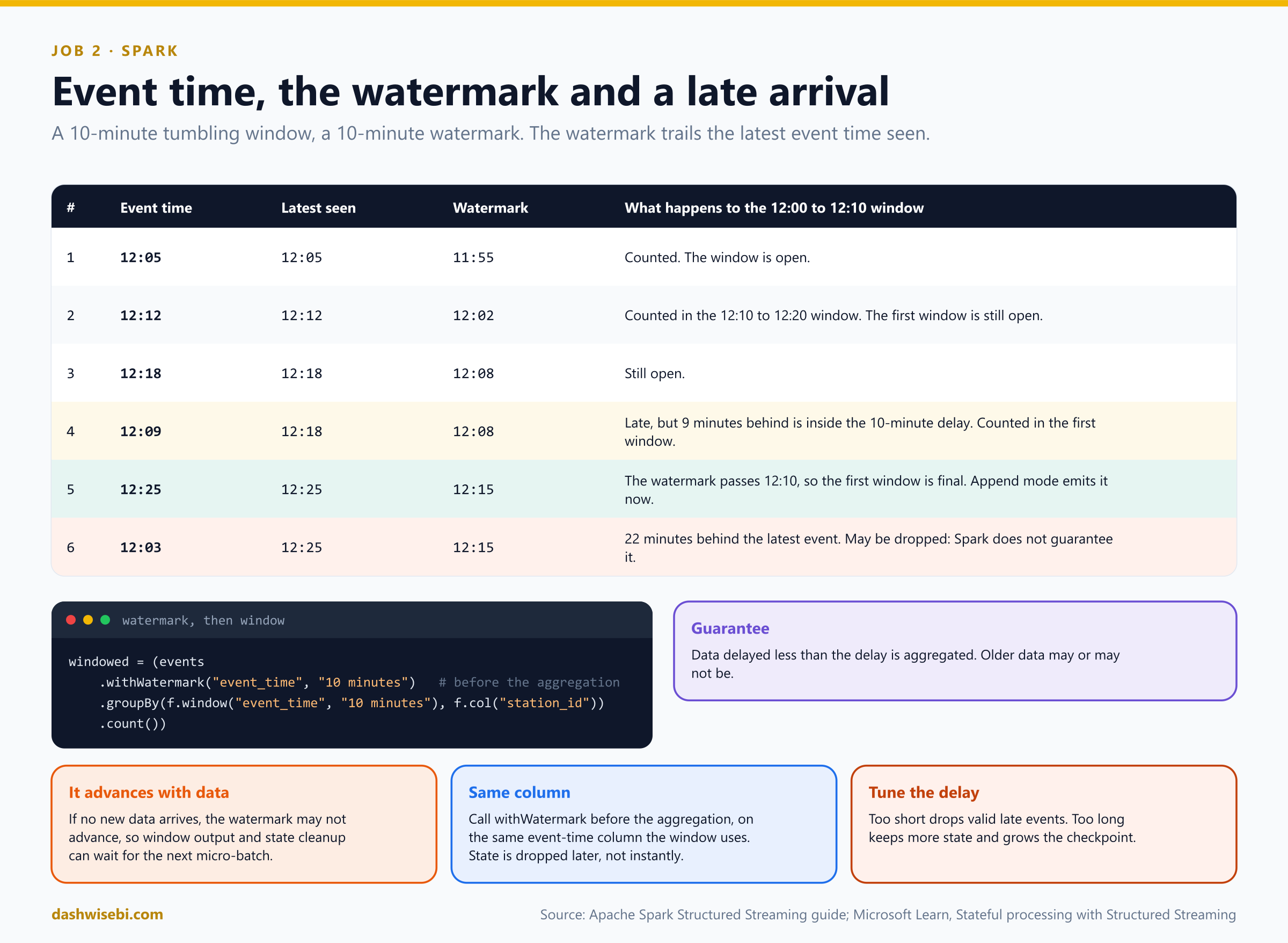
Pause and decide. You set a watermark of 10 minutes. The latest event time seen is 12:18. What is the watermark, and what happens to a ping from 12:09?
The watermark is 12:08, the latest event time minus the delay. A ping from 12:09 is 9 minutes behind, inside the 10-minute delay, so it is aggregated. Data delayed less than the threshold is guaranteed to be aggregated. Data delayed more may or may not be.
Pause and decide. The same job later sees an event from 12:25. When does the 12:00 to 12:10 window appear in Append mode?
When the watermark passes the window end. With a latest event time of 12:25 the watermark is 12:15, past 12:10, so the window is final and Append mode emits it. A later ping from 12:03 is 22 minutes behind and may be dropped.
Pause and decide. The stadium stream goes quiet for ten minutes, and the dashboard shows nothing new for the last window. Bug?
Not necessarily. The watermark advances when new data arrives. If nothing arrives, window output, unmatched outer-join rows and state cleanup can wait until a later micro-batch receives data.
clean = (events
    .withWatermark("event_time", "10 minutes")
    .dropDuplicatesWithinWatermark(["event_id"]))

counts = (clean
    .groupBy(
        f.window("event_time", "5 minutes"),
        f.col("station_id"))
    .count())

(counts.writeStream
    .format("delta")
    .outputMode("append")
    .option("checkpointLocation", "Files/checkpoint_counts")
    .toTable("station_5min"))
Why: state is memory, so bound it
Pause and decide. Which is correct for removing resent pings: (a) dropDuplicates(["event_id"]) on its own, or (b) withWatermark plus dropDuplicatesWithinWatermark(["event_id"])?
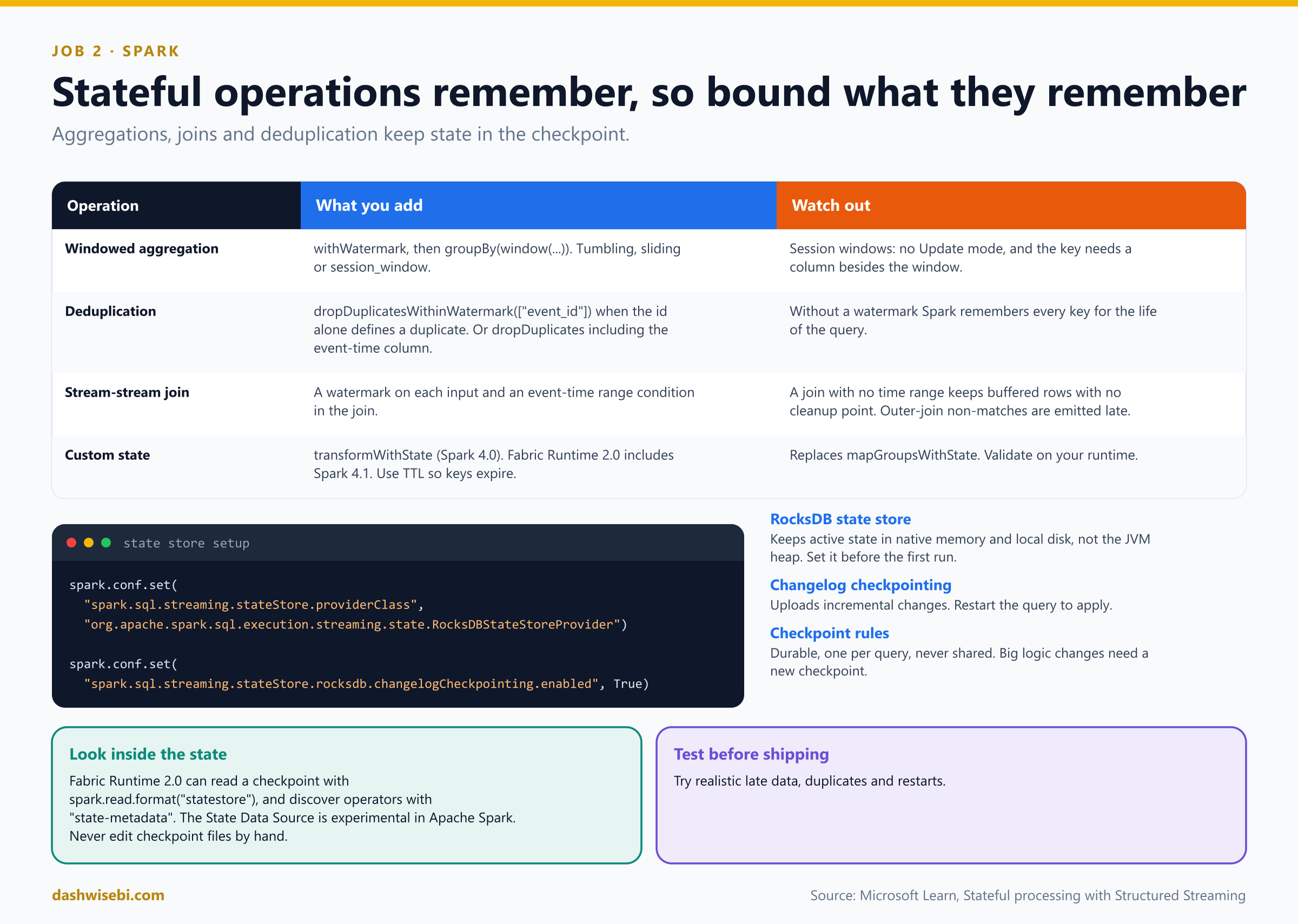
(b) when the id alone defines a duplicate. Without a watermark, dropDuplicates must remember every key for the life of the query. To let Spark evict the old state with the older API, include the watermark column in the key (["event_id", "event_time"]), which means two records with the same id but different timestamps are not duplicates.
Pause and decide. Imran wants to join the ping stream with a stream of lock events by bike id. What stops state from growing forever?
A watermark on each input and an event-time range condition in the join, for example the lock event must be within five minutes of the ping. With no time range, Spark must keep buffered rows with no cleanup point. For outer joins, unmatched rows are emitted only when the watermark proves no future match can arrive.
Pause and decide. The aggregation state is large and the executors are under memory pressure. What do you change?
Switch the state store to RocksDB, which keeps active state in native memory and on local disk instead of the JVM heap: set spark.sql.streaming.stateStore.providerClass to org.apache.spark.sql.execution.streaming.state.RocksDBStateStoreProvider before the query's first run. Add changelog checkpointing (spark.sql.streaming.stateStore.rocksdb.changelogCheckpointing.enabled) to reduce checkpoint latency, and restart the query for it to take effect.
- Checkpoint rules. Use a durable location. Never share one checkpoint between different queries. Major changes to stateful logic often need a new checkpoint.
- Custom state logic uses
transformWithState, which replacesmapGroupsWithStateandflatMapGroupsWithState. It arrived in Spark 4.0, and Fabric Runtime 2.0 includes Spark 4.1. Use TTL so keys expire. - Inspect state with
spark.read.format("statestore")on Runtime 2.0 or later. It is experimental in Apache Spark. Never edit checkpoint files by hand. - Choose the delay from real source behavior. Too short drops valid late data. Too long keeps more state and grows the checkpoint.
Priya refreshes the dashboard. The stadium counts now match the trip totals, and the resent pings are gone. “How late is too late?” she asks. You show her the watermark and the 10-minute delay. “That is a business decision,” you say. “I will help you choose it.”
Exam lens
- Event time versus arrival time. Watermark = latest event time minus the delay. Call
withWatermarkbefore the aggregation, on the same column. - Append emits a window after the watermark passes its end. The watermark moves only when data arrives.
- Deduplicate with a watermark. Join streams with watermarks and a time range. RocksDB for big state.
- Session-window aggregations do not support Update mode.
Chapter 3. Sunil: I do not want to wait for Spark
Sunil leans on the desk. “My dashboards need clean columns the moment a ping lands, and per-minute counts per station. I do not want a Spark job for that. The Eventhouse can do it.”
He is right. The Eventhouse is built to shape and answer on arrival, with KQL and two features you saw in Episode 7: update policies and materialized views. In streaming scenarios the details matter.
Pause and decide. Raw pings arrive in a single string column. You want typed columns in another table, automatically, as data lands. Which feature?
An update policy. It is triggered when new data is written to a source table, runs a query to transform it, and saves the result in a target table, with no extra orchestration. The target can have a different schema and retention policy.
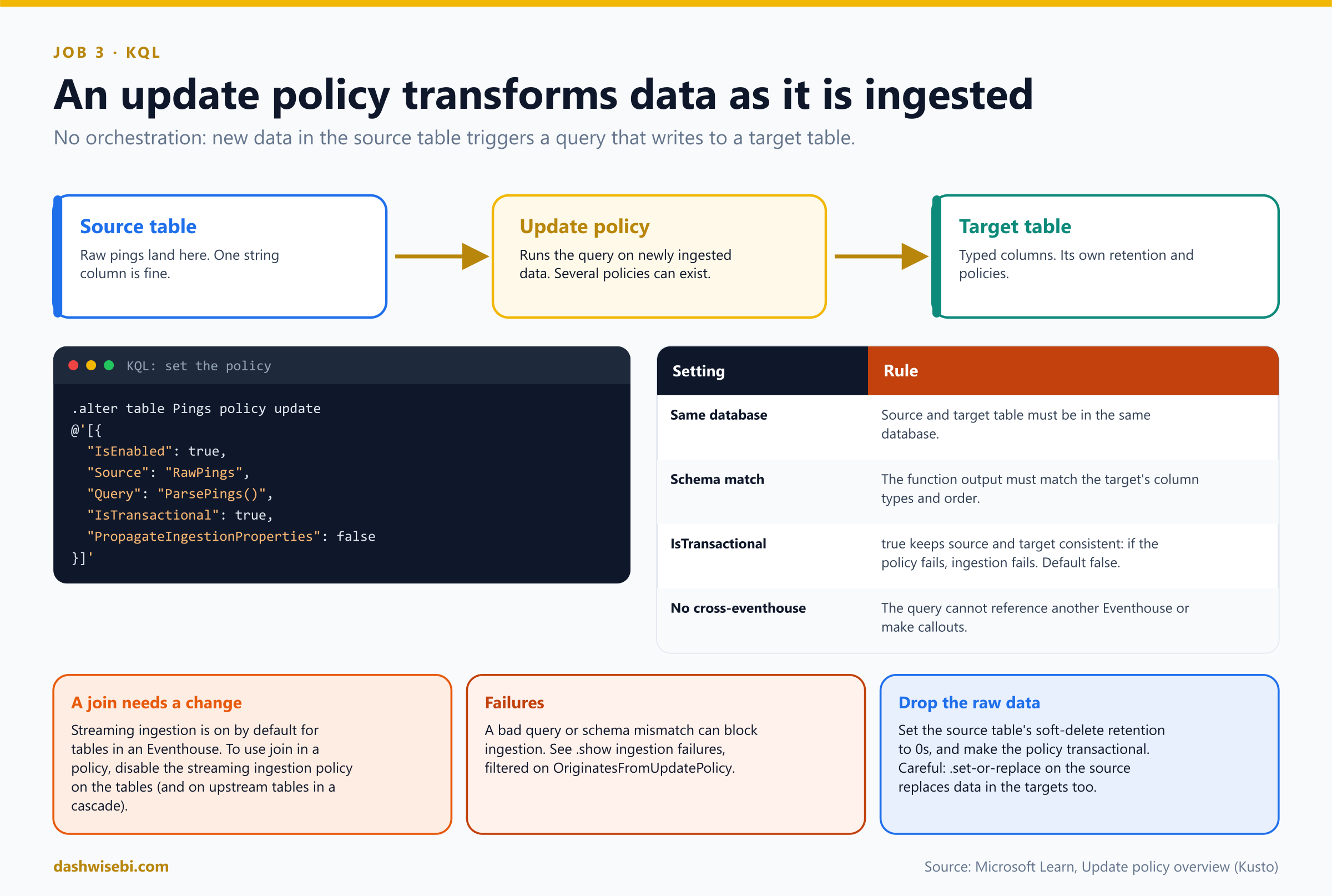
.create table RawPings (Raw: string)

.create table Pings (Timestamp: datetime, BikeId: string, Station: string, Event: string)

.create function with (docstring = "Parse raw pings", folder = "UpdatePolicyFunctions") ParsePings()
{
    RawPings
    | extend j = parse_json(Raw)
    | project Timestamp = todatetime(j.ts), BikeId = tostring(j.bike),
              Station = tostring(j.station), Event = tostring(j.event)
}

.alter table Pings policy update
@'[{ "IsEnabled": true, "Source": "RawPings", "Query": "ParsePings()", "IsTransactional": true, "PropagateIngestionProperties": false }]'
Pause and decide. The function's output columns are in a different order than the target table's columns. What happens?
It fails. The update policy function's schema and the target table's schema must match in column types and order. An incorrect query or schema mismatch can block ingestion into the source table, so test the function first.
Pause and decide. What does IsTransactional: true change, and what does Microsoft recommend for production?
With false (the default), if the policy fails, data is ingested to the source table only, and the ingestion itself still succeeds. With true, consistency between the source and target is guaranteed: if the policy fails, data is ingested to neither table and the ingestion fails. Microsoft's note says to set it to true in production so the target does not lose data in transient failures.
Pause and decide. Sunil wants to keep only the parsed data and not store the raw table for long. How?
Set the source table's soft-delete retention to 0s and make the update policy transactional. Then the source data is not queryable and not stored durably after ingestion. A caution: running .set-or-replace on the source replaces data in derived tables too, so consider .set-or-append.
Pause and decide. Your update policy function uses a join to add station names and ingestion starts failing. What is a known cause in an Eventhouse?
The streaming ingestion policy is enabled by default for tables in an Eventhouse. To use a function with a join in an update policy, that policy must be disabled. For cascading update policies (table A feeds B feeds C), disable it on all upstream tables.
- Same database. Source and target tables must be in the same database. The query cannot reference another Eventhouse or make callouts.
- See failures with
.show ingestion failures, filtered onOriginatesFromUpdatePolicy. - Several policies can exist on one table, and cascades are allowed. Circular ones are cut at runtime.
- Preview: the source of an update policy can also be an external delta table that has a query acceleration policy, for example a OneLake shortcut from Episode 10. It runs asynchronously, ignores deletes on the source, and cannot be transactional.
Materialized views: the always-fresh aggregate
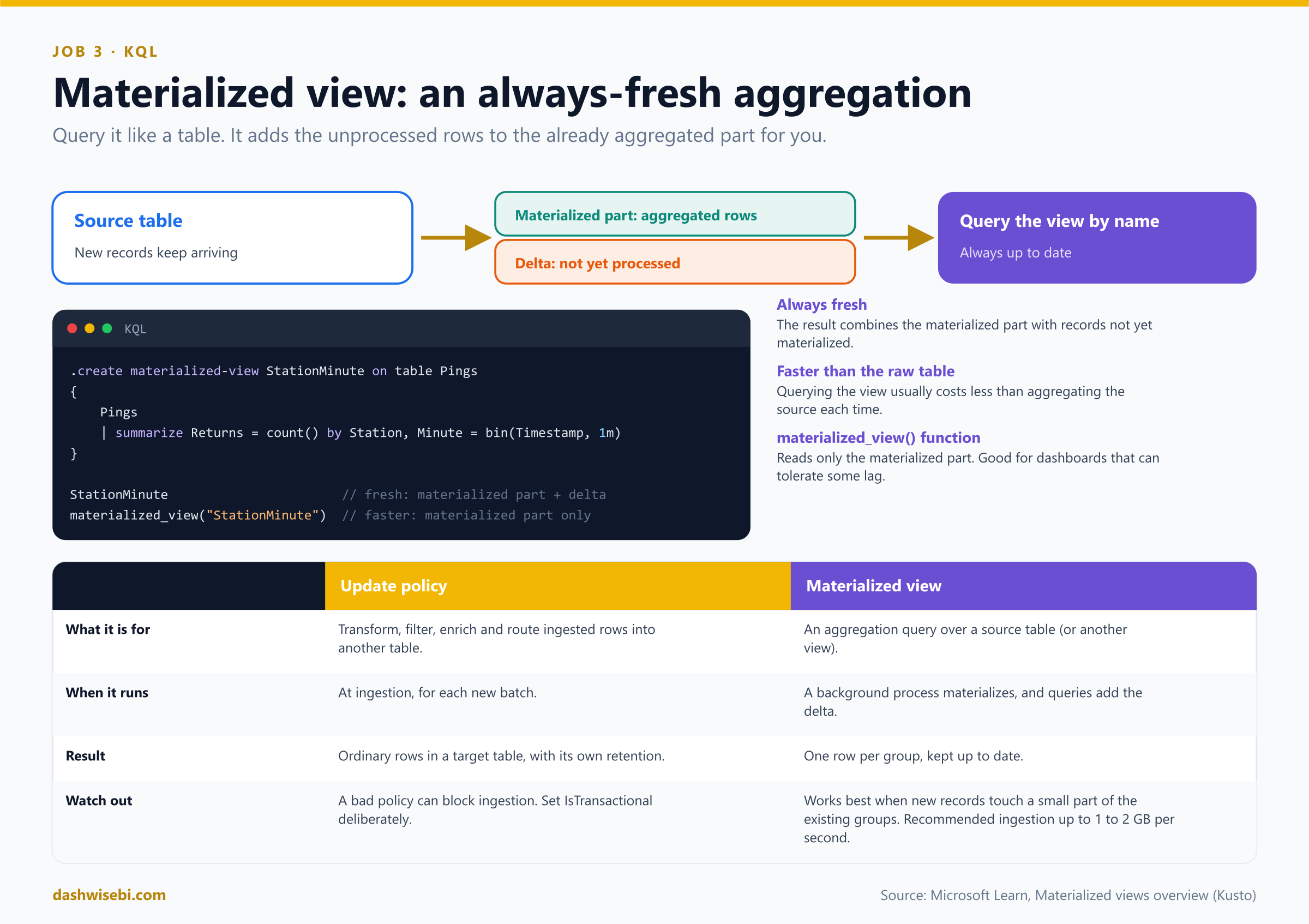
.create materialized-view StationMinute on table Pings
{
    Pings
    | summarize Returns = count() by Station, Minute = bin(Timestamp, 1m)
}

StationMinute                         // fresh: materialized part + delta
materialized_view("StationMinute")    // faster: materialized part only
Pause and decide. A dashboard must show per-minute counts as fast as possible and can tolerate a little lag. How do you query the view?
With the materialized_view() function. It reads only the materialized part, so it is always faster than querying the whole view, but it is not guaranteed to include the latest records. Querying the view by name combines the materialized part with the delta and is always up to date.
Pause and decide. Which fits better: an update policy or a materialized view? (a) Parse and filter pings into a typed table. (b) Keep a running count per station per minute.
(a) is an update policy: transform, filter, enrich and route rows. (b) is a materialized view: an aggregation that stays fresh. They work well together: the update policy fills a typed table, and a view aggregates it.
- A view works best when new records touch a small part of the existing groups. If most groups change on every cycle, materialization suffers. The recommended ingestion rate is up to 1 to 2 GB per second.
- A view over another view needs the source view to be a deduplication view (
take_any(*)). - A materialized view reduces the cost of querying, and you can reduce the source table's retention when only the aggregation is needed.
Querying by time: bin, make-series and sessions
Pause and decide. Some five-minute windows have no returns. In a summarize ... by bin(Timestamp, 5m) result, what do those windows look like?
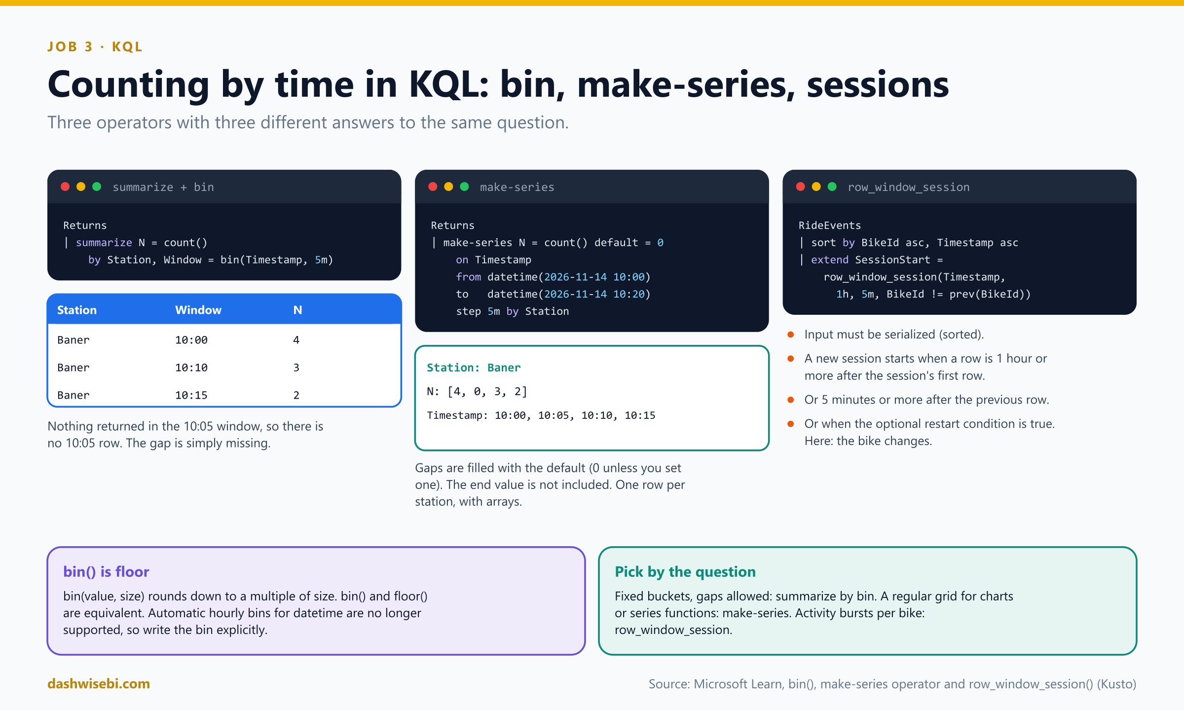
They are missing. summarize returns one row for each group that has data. For a regular time grid with zeros, use make-series, which fills gaps with a default (0 unless you set one) and returns arrays. Its to value is not included.
// one row per station and window that has data
Returns
| summarize N = count() by Station, Window = bin(Timestamp, 5m)

// one row per station, arrays with a value for every step
Returns
| make-series N = count() default = 0
    on Timestamp from datetime(2026-11-14 10:00) to datetime(2026-11-14 10:20) step 5m
    by Station
Pause and decide. What is bin(Timestamp, 5m), and what happened to the automatic hourly bins that older queries relied on?
bin(value, roundTo) rounds a value down to a multiple of the bin size (it is equivalent to floor()). Automatic hourly bins for datetime columns in summarize are no longer supported, so always write the bin explicitly.
Pause and decide. Karan wants each bike's rides grouped into sessions: a new session after 5 quiet minutes, or when it passes an hour, or when the bike changes. Which function?
row_window_session() over a sorted (serialized) row set. It returns the start value of each session. A new session begins when a row is at least MaxDistanceFromFirst after the session's first row, at least MaxDistanceBetweenNeighbors after the previous row, or when the optional Restart condition is true.
RideEvents
| sort by BikeId asc, Timestamp asc
| extend SessionStart = row_window_session(Timestamp, 1h, 5m, BikeId != prev(BikeId))
| summarize Events = count(), SessionEnd = max(Timestamp) by BikeId, SessionStart
Sunil runs the dashboard query against the materialized view. It returns in a blink, with a count that includes a ping that landed two seconds ago. “No Spark job,” he says, satisfied.
Exam lens
- Update policy: transform on ingestion. Same database, matching schema, IsTransactional true for production, streaming ingestion must be off for joins.
- Materialized view: always-fresh aggregate.
materialized_view()reads the materialized part only. - summarize by bin skips empty bins. make-series fills them. row_window_session needs sorted input.
Chapter 4. Karan: the busiest five minutes, and how long a session lasts
It is almost noon and the Cyclothon crowd is thinning. Karan finally sits down. “Three things. The busiest five minutes at each station. An alert when a station sees too many returns in a rolling window. And how long each ride session lasts.”
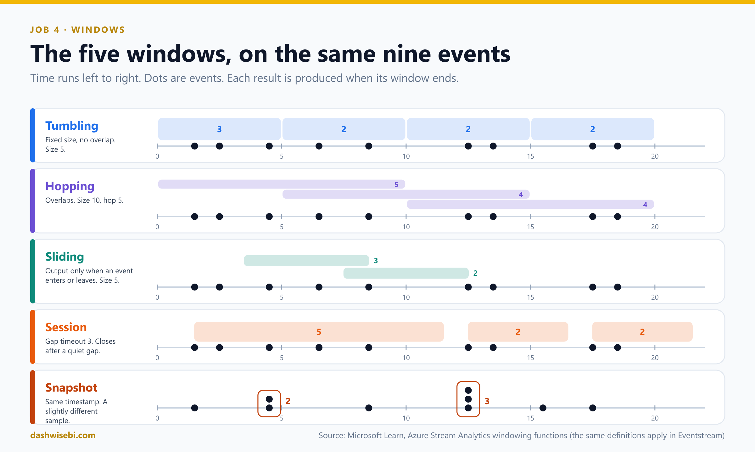
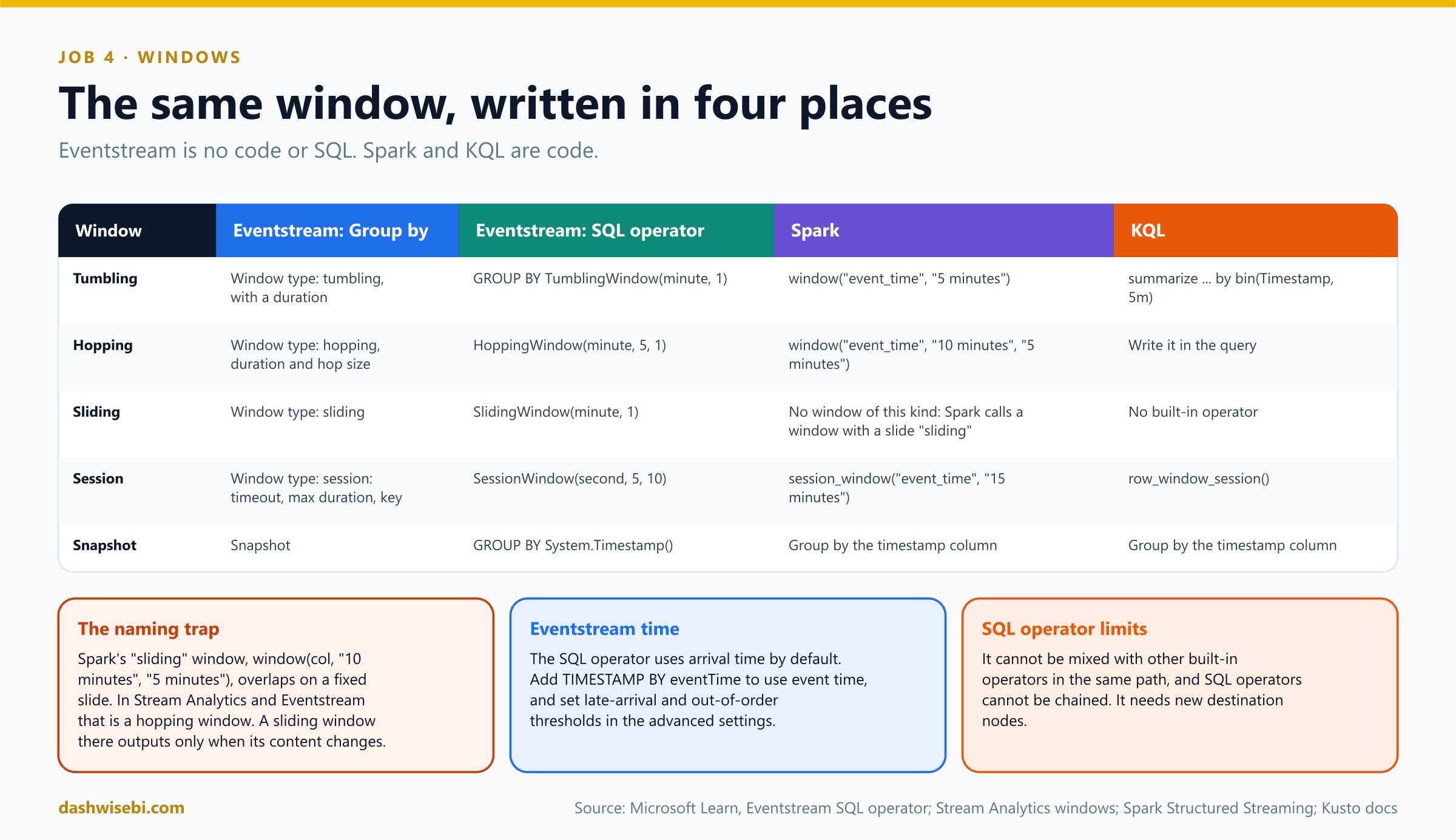
These are all windowing functions: they group events by time before they aggregate. There are five kinds, and the same ones appear in Eventstream, Azure Stream Analytics and (with different names) in Spark and KQL.
Pause and decide. “The busiest five minutes at each station.” Which window?
Tumbling. Fixed-size, contiguous, non-overlapping windows. An event belongs to exactly one window, so each five-minute period gets exactly one count.
Pause and decide. “A rolling 10 minutes of returns, evaluated every minute, to flag a station that is emptying.” Which window and which parameters?
Hopping, with a window size of 10 minutes and a hop of 1 minute. A hopping window is a tumbling window that can overlap and be emitted more often than its size. An event can belong to several hopping windows. A tumbling window is just a hopping window whose hop equals its size.
Pause and decide. “How long does each bike's ride session last?” Which window, and what must you configure?
Session. A session starts with the first event and extends as long as the next event arrives within the timeout. If events keep arriving, it extends until the maximum duration. An optional partitioning key (here the bike id) gives each bike its own sessions.
Pause and decide. What is a sliding window, and how does it differ from hopping?
A sliding window outputs a result only when its content changes, that is, when an event enters or leaves the window. So every output window has at least one event. A hopping window outputs on a fixed schedule even if nothing changed.
Pause and decide. What does a snapshot window group, and how do you write it?
Events that have the same timestamp. You do not call a window function. You add System.Timestamp() to the GROUP BY clause.
Why: one result per window, at the end of the window
- All of these windowing operations output their result at the end of the window. The output event carries the timestamp of the window end.
- In Eventstream, the SQL operator uses arrival time by default. To use event time, add
TIMESTAMP BYin the query. You can also set thresholds for late-arriving and out-of-order events in the SQL operator's advanced settings. - The Azure Stream Analytics documentation (the query language Eventstream builds on) notes a maximum window size of 7 days.
In Eventstream
The Group by transformation calculates aggregations across events in time windows. Microsoft's training module names tumbling and sliding windows for it, and the Eventstream definition format also lists hopping, session and snapshot windows, so check the Group by pane in your tenant for what it offers today. For full control, add a SQL operator, which uses the Stream Analytics query language. Here are RideWise's three questions as SQL:
-- busiest five minutes per station (tumbling), by event time
SELECT System.Timestamp() AS WindowEnd, stationId, COUNT(*) AS Returns
INTO StationFiveMinutes
FROM Pings TIMESTAMP BY eventTime
GROUP BY stationId, TumblingWindow(minute, 5)

-- too many returns in a rolling 10 minutes, evaluated every minute (hopping)
SELECT System.Timestamp() AS WindowEnd, stationId, COUNT(*) AS Returns
INTO Alerts
FROM Pings TIMESTAMP BY eventTime
GROUP BY stationId, HoppingWindow(minute, 10, 1)
HAVING COUNT(*) > 40

-- ride sessions per bike: 5 minute timeout, 60 minute maximum
SELECT bikeId, MIN(eventTime) AS SessionStart, System.Timestamp() AS SessionEnd
INTO RideSessions
FROM Pings TIMESTAMP BY eventTime
GROUP BY bikeId, SessionWindow(minute, 5, 60)
Each statement writes to its own output, and a single SQL operator can fan out to several destinations with several INTO clauses. Read the input once with a WITH clause when you reuse it.
Pause and decide. Priya adds a SQL operator to an eventstream that already has a Filter operator in the same path. What does she find?
A limit. The SQL operator is designed to centralize all your transformation logic, so you cannot use it alongside other built-in operators within the same processing path, and you cannot chain SQL operators. You also need to create new destination nodes for it, and the eventstream name must not contain an underscore or a dot.
In Spark
# tumbling: no slide argument
f.window("event_time", "5 minutes")

# overlapping, every 1 minute (what Stream Analytics calls hopping)
f.window("event_time", "10 minutes", "1 minute")

# session: closes after a 5 minute gap
(events.withWatermark("event_time", "10 minutes")
    .groupBy(f.session_window("event_time", "5 minutes"), f.col("bike_id"))
    .count())
Pause and decide. The Spark documentation calls window(col, "10 minutes", "1 minute") a sliding window. How does that match the Eventstream window names?
It is what Stream Analytics and Eventstream call a hopping window: a fixed size that overlaps because the slide is smaller than the size. The Eventstream sliding window is a different thing that outputs only when its content changes. Watch for this on the exam.
Pause and decide. A Spark session-window aggregation must run in Update mode to show running results. Is that allowed?
No. For streaming session-window aggregations, Update output mode is not supported. The grouping key must also include at least one column besides session_window. Use Append (with a watermark) or Complete.
In KQL
KQL has no TumblingWindow keyword. A tumbling window is summarize ... by bin(Timestamp, 5m), and a regular grid is make-series. Sessions are row_window_session(). I did not find a built-in overlapping-window operator on the pages I used, so for hopping and sliding windows in KQL you write the logic in the query. Treat this as the one place where KQL is more manual than the stream engines.
By one o'clock Karan has his three answers: five-minute counts, a ten-minute alert that fires every minute, and session lengths per bike. The dashboard has a new tile, and the station near Baner shows red, three bikes from empty. A van is already on its way.
Exam lens
- Tumbling = fixed, no overlap. Hopping = size plus hop, overlaps. Sliding = output when content changes. Session = timeout, max duration, optional key. Snapshot = same timestamp,
System.Timestamp(). - Results come at the end of the window, with the window-end timestamp.
- Spark naming trap:
window(col, size, slide)is hopping. - KQL: bin for tumbling,
row_window_sessionfor sessions. Eventstream SQL operator: arrival time by default,TIMESTAMP BYfor event time, no mixing with other built-in operators.
The review: ten quick calls
At two o'clock the four of them are back at your desk with the same question: did we choose well? Answer in your head first, then open each one.
Pause and decide. 1. A streaming job must restart itself after an infrastructure failure. What do you configure?
Run it as a Spark job definition and turn on the retry policy. It has a lifetime limit of 90 days.
Pause and decide. 2. Which settings make a streaming Delta write produce larger files?
A processingTime trigger and Optimized Write (and sensible partitioning).
Pause and decide. 3. Which output mode can a windowed aggregation with a watermark use, and when does Append emit a window?
Append, Update or Complete. Append emits a window after the watermark passes the window end.
Pause and decide. 4. How do you remove resent events by id without unbounded state?
withWatermark plus dropDuplicatesWithinWatermark.
Pause and decide. 5. Name the setting that reduces Spark state memory pressure.
The RocksDB state store provider, with changelog checkpointing for faster checkpoints.
Pause and decide. 6. What triggers an update policy, and where must the source and target tables be?
New data ingested into the source table. Both tables must be in the same database.
Pause and decide. 7. Which materialized view query returns only the already processed rows?
materialized_view("Name").
Pause and decide. 8. Which KQL operator returns a value for every time step, including empty ones?
make-series with a default value.
Pause and decide. 9. A window that closes after a quiet period and has a maximum duration. Which window and which parameters?
A session window: timeout, maximum duration and an optional partition key.
Pause and decide. 10. Which window is Spark's window(col, "10 minutes", "1 minute") in Eventstream terms?
A hopping window.
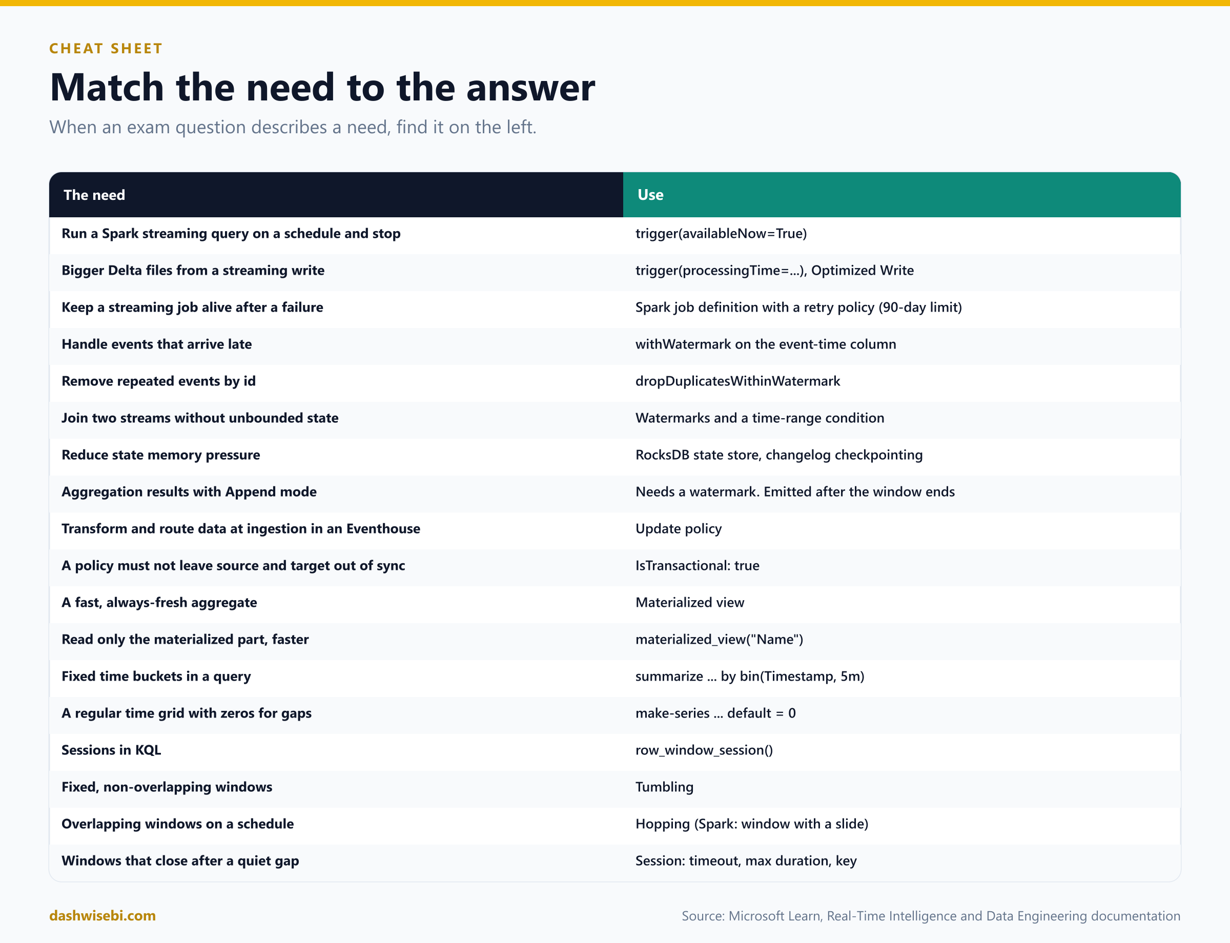
The cheat sheet
Myth or fact?
- “Run production streaming from a notebook.” Myth. Use a Spark job definition with a retry policy.
- “The retry policy lasts forever.” Myth. It has a lifetime limit of 90 days.
- “Append mode works for any aggregation.” Myth. Aggregations need a watermark for Append.
- “The watermark advances with the clock.” Myth. It advances when new data arrives.
- “Data later than the watermark is always dropped.” Myth. It may be processed, but Spark does not guarantee it.
- “One checkpoint can serve many queries.” Myth. One checkpoint per query.
- “An update policy can read from another Eventhouse.” Myth. It cannot make cross-eventhouse queries.
- “A non-transactional update policy blocks ingestion on failure.” Myth. Only a transactional one does. The default is non-transactional.
- “summarize by bin returns empty windows.” Myth. Use make-series for that.
- “Spark's sliding window is Eventstream's sliding window.” Myth. It is a hopping window.
- “The SQL operator can be mixed with other operators.” Myth. It cannot be used alongside other built-in operators in the same path.
Where to go next
- Run the
rate-source job from the quickstart as a Spark job definition. Turn the retry policy on, stop it, and look at the Structured Streaming tab in the monitoring hub. - Write a tumbling count with a 10-minute watermark. Feed it events with timestamps out of order and watch when Append emits each window.
- In an Eventhouse, create
RawPings,Pings, the function and the update policy from this post. Then break the function's column order on purpose, and read.show ingestion failures. - Create the
StationMinuteview and compare querying it by name withmaterialized_view(). - Add a SQL operator to an eventstream, and write the same question as a tumbling, a hopping and a session window.
- Read the sources behind this post: DP-700 study guide, Data streaming into a lakehouse with Spark, Get started with streaming data in lakehouse, Stateful processing with Structured Streaming, Apache Spark: Structured Streaming operations on DataFrames, Update policy overview, Materialized views overview, bin(), make-series operator, row_window_session(), Process events using a SQL operator, Eventstream transformations and Stream Analytics windowing functions.
Keep reading
DP-700 Episode 10: Streaming I, Engines & Eventstream
DP-700 study guide told as a story: pick a streaming engine, choose native tables or shortcuts, decide on query acceleration, and build an Eventstream.
DP-700 Episode 7: Batch Transformation with PySpark, SQL & KQL
DP-700 study guide to batch transformation in Fabric with PySpark, T-SQL and KQL: denormalizing, aggregating, and handling duplicate, missing and late data.