PL-300 Episode 3: Design the Data Model

Welcome to Episode 3 of our PL-300 series. In Part 1 we connected to data and profiled it. In Episode 2 we cleaned it in Power Query and shaped it into fact tables and dimension tables. Now the tables are loaded, and the real modelling begins.

This episode opens the Model the data skill area (25 to 30 percent of the exam) with the group Design and implement a data model. These are the five skills:

• Configure table and column properties
• Implement role-playing dimensions
• Define a relationship's cardinality and cross-filter direction
• Create a common date table
• Identify use cases for calculated columns and calculated tables

Along the way we also cover the star schema, the snowflake schema and the galaxy schema with ER diagrams, active and inactive relationships, limited relationships, why many-to-many is risky, and when to use a single or a both-way filter. Every idea comes with a small data example, and the date table, calculated columns and calculated tables come with both Power Query M and DAX code you can copy.

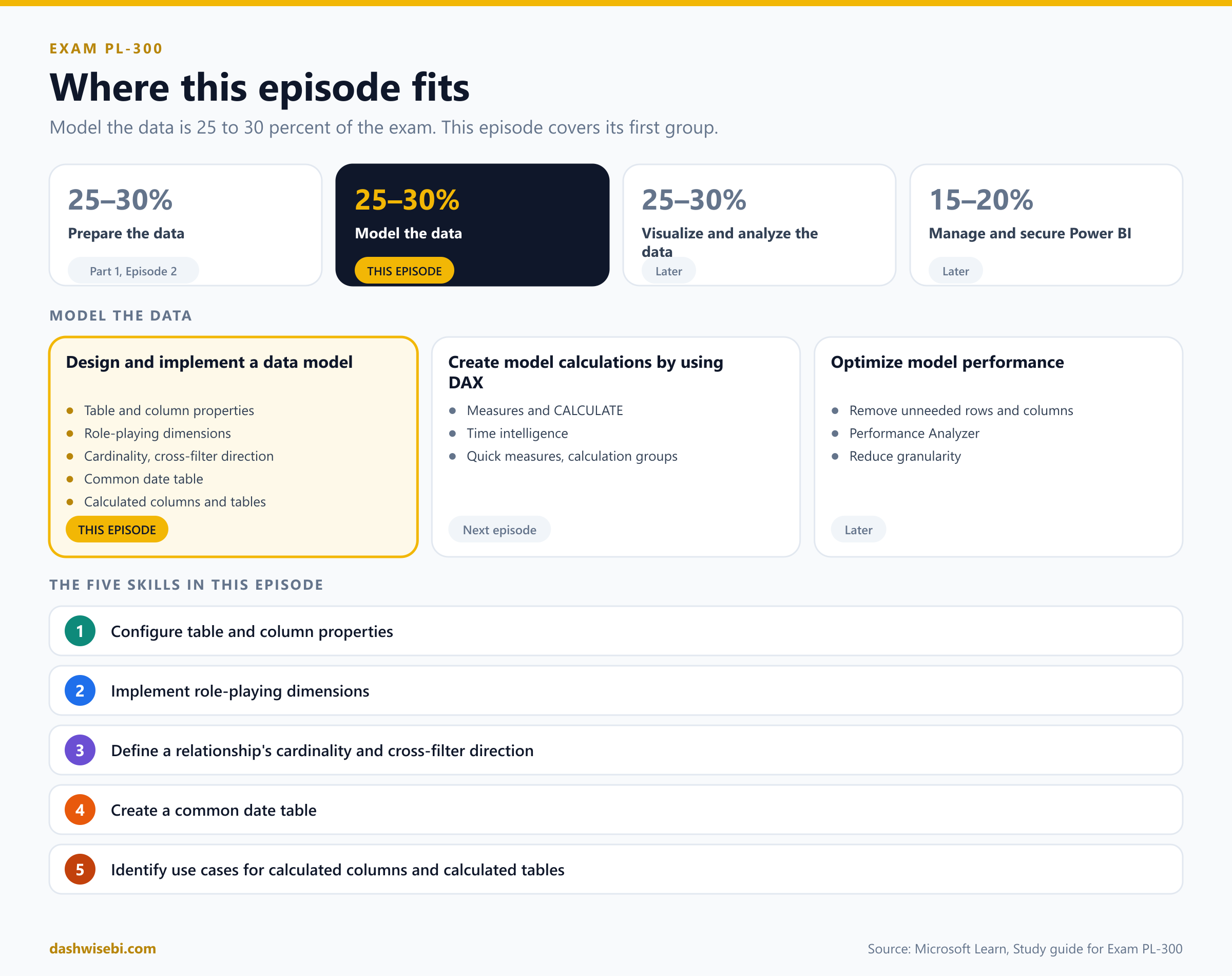
A note on wording. The study guide Microsoft updated on 5 November 2026 (skills measured as of 20 April 2026) lists these five bullets under Design and implement a data model. The next group, Create model calculations by using DAX, also mentions calculated tables and columns. Here we focus on when to use them in a model, and show the syntax. The DAX group continues in the next episode.

---

The big picture: tables, relationships, calculations

A Power BI semantic model is three things working together. Tables hold the data. Relationships decide how a filter on one table reaches another. Calculations (measures, calculated columns and calculated tables) add logic. Most exam questions in this area ask one thing: if the user filters here, what happens over there?

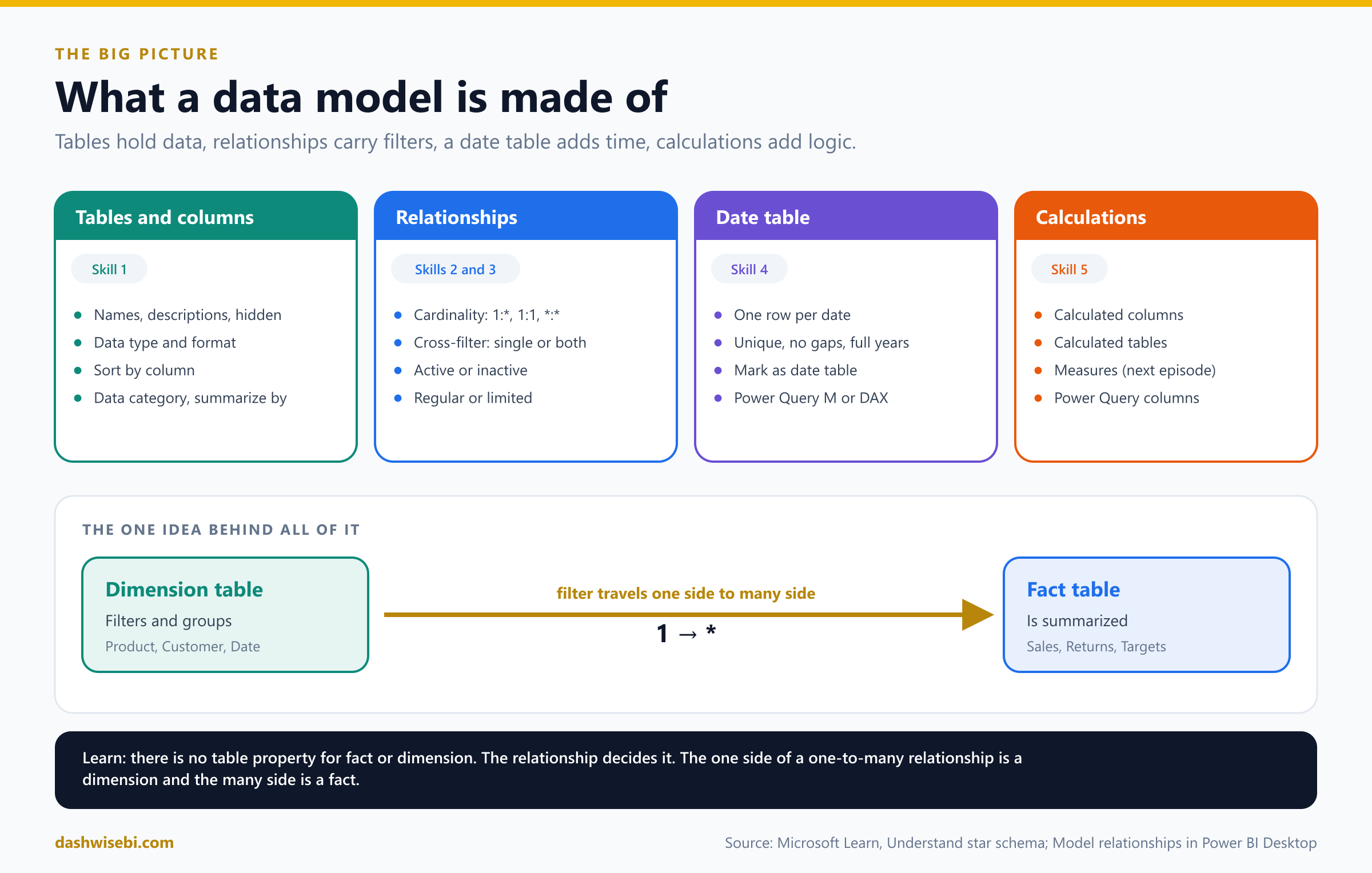
Keep one picture in your head: dimension tables filter and group, fact tables summarize, and a relationship is the road a filter travels from a dimension to a fact. Learn says there is no table property that marks a table as a dimension or a fact. The relationship decides it: the "one" side of a one-to-many relationship is a dimension and the "many" side is a fact.

---

Star, snowflake and galaxy schemas

Before the five skills, you need a layout in mind. Three layouts come up again and again.

Star schema

A star schema has one fact table in the middle and dimension tables around it, each related to the fact table with a one-to-many relationship. It is the layout Microsoft recommends for Power BI.

• Dimension tables describe the things you model: products, customers, places, time. They have a unique key column and attribute columns used to filter and group. They usually have relatively few rows.
• Fact tables store observations or events: sales, stock balances, temperatures. They hold dimension key columns and numeric columns to summarize. They can have many rows and keep growing.
• The dimension key columns set the dimensionality of the fact table. The key values set its granularity. A target table keyed by the first day of each month and by product has a grain of month and product.
• A fact table should always load at one consistent grain. Do not mix dimension and fact columns in one table.

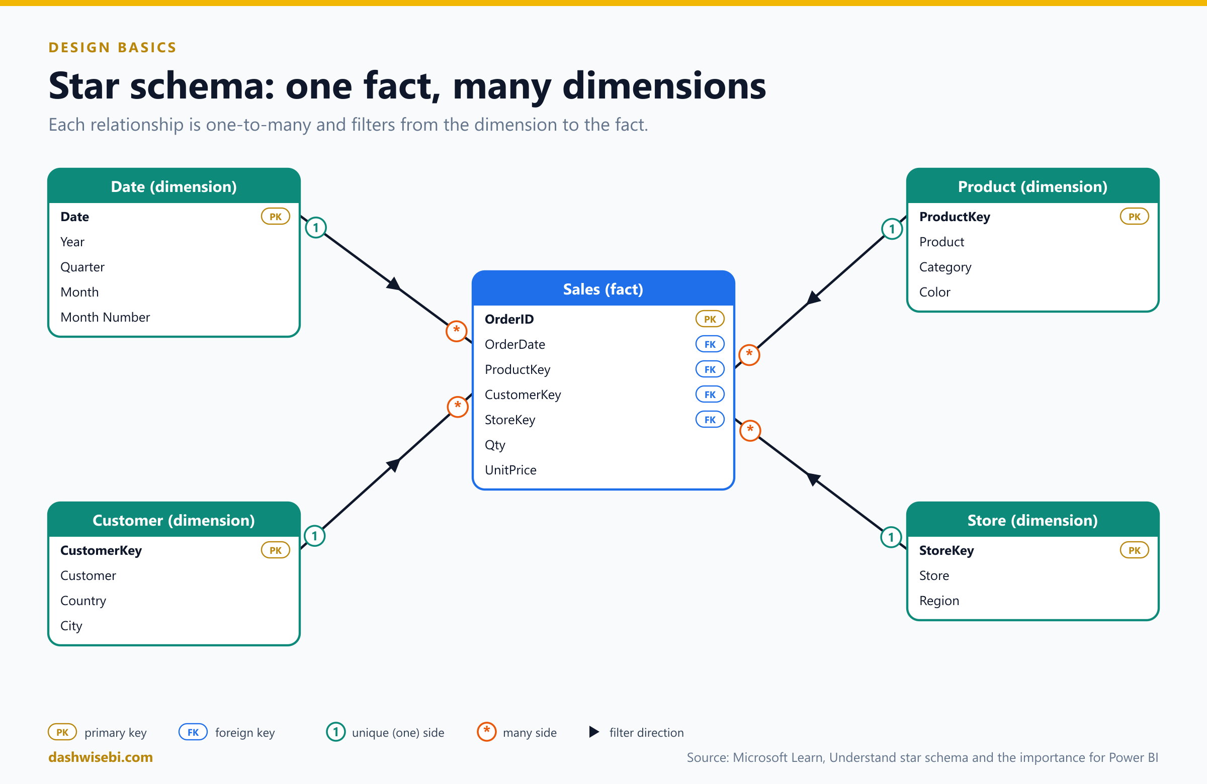
Here is a small example you will see again later. One dimension (Product) and one fact (Sales):

Product (dimension: one row per product)
ProductKey | Product   | Category    | Color
1          | Road Bike | Bikes       | Red
2          | Helmet    | Accessories | Blue
3          | Lock      | Accessories | Blue
4          | Cap       | Accessories | Red

Sales (fact: one row per order)
OrderID | OrderDate  | ShipDate   | ProductKey | CustomerKey | Qty | UnitPrice
1001    | 2026-01-05 | 2026-01-08 | 1          | 10          | 1   | 900
1002    | 2026-01-20 | 2026-01-22 | 2          | 20          | 2   | 40
1003    | 2026-02-03 |            | 2          | 10          | 1   | 40
1004    | 2026-02-14 | 2026-02-18 | 3          | 30          | 1   | 25

The Sales table stores only the key ProductKey, not the product's name or color. Storing only keys in the fact table is called normalized. Storing the name, category and color in the fact table too would be denormalized. A star schema keeps the fact table normalized and makes each dimension table wide and flat, with every attribute in one table.

Snowflake schema

A snowflake schema normalizes a dimension into several related tables. The classic example: products belong to subcategories, and subcategories belong to categories, so the product dimension becomes three tables in a chain.

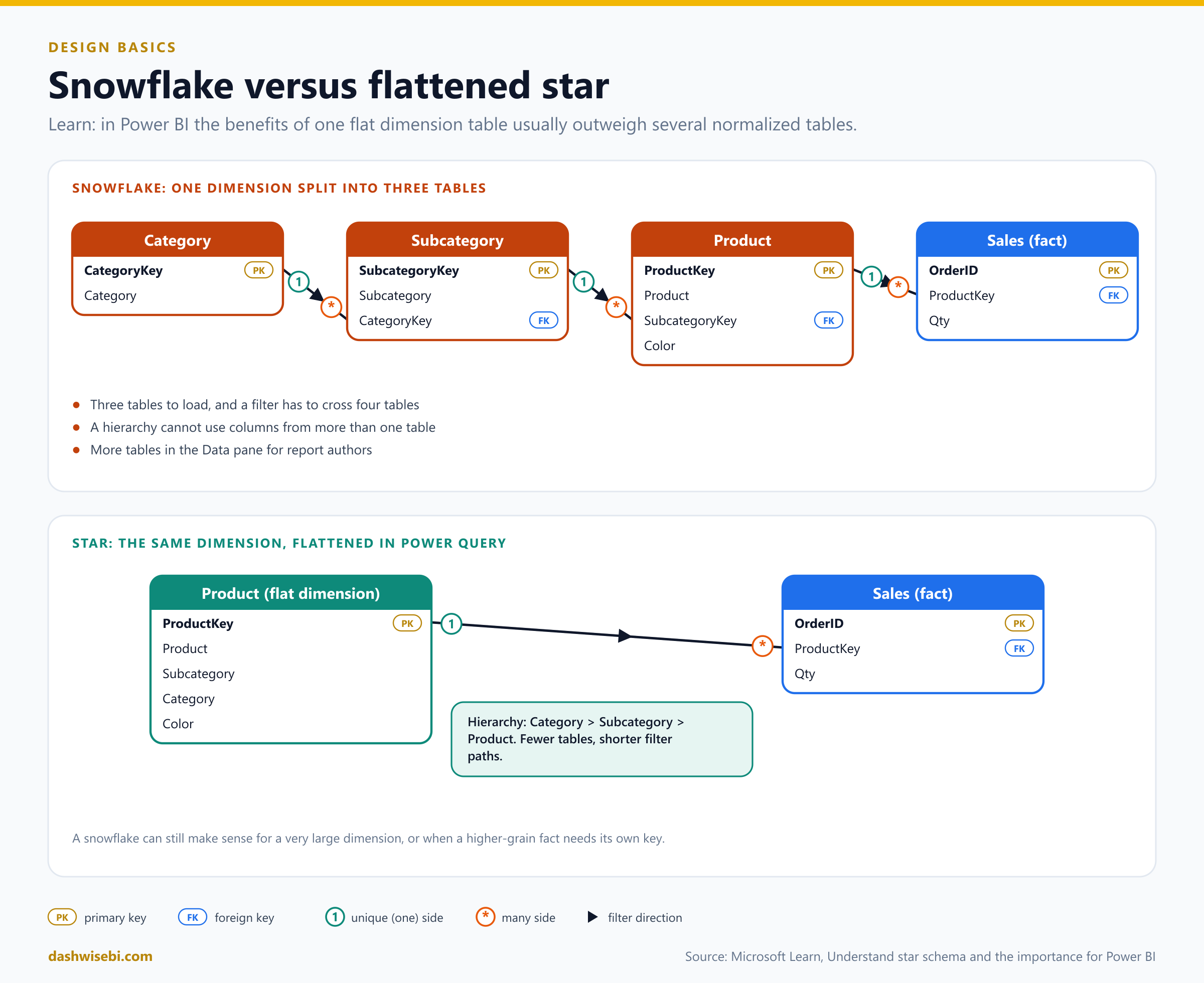
Power BI lets you mimic a snowflake, but Learn says the benefits of one flat table usually outweigh the benefits of several. With a snowflake:

• Power BI loads more tables, which is less efficient for storage and speed, and the model can grow.
• Filters must travel along longer chains of relationships.
• The Data pane shows more tables, which is less friendly, especially for tables with one or two columns.
• You cannot build a hierarchy from columns in different tables.

Flattening has one cost: redundant text is stored in the dimension. For most dimensions that is a small price. A snowflake can still make sense when the dimension is very large and storage matters more than speed, when a higher-grain fact (like targets by subcategory) needs its own key, or when you must track history at a higher level.

To flatten a snowflake in Power Query, merge the tables (Episode 2) and remove the helper keys:

let
    WithSub = Table.NestedJoin(Product, {"SubcategoryKey"}, Subcategory, {"SubcategoryKey"}, "Sub", JoinKind.LeftOuter),
    ExpSub  = Table.ExpandTableColumn(WithSub, "Sub", {"Subcategory", "CategoryKey"}),
    WithCat = Table.NestedJoin(ExpSub, {"CategoryKey"}, Category, {"CategoryKey"}, "Cat", JoinKind.LeftOuter),
    ExpCat  = Table.ExpandTableColumn(WithCat, "Cat", {"Category"}),
    Flat    = Table.RemoveColumns(ExpCat, {"SubcategoryKey", "CategoryKey"})
in
    Flat

Then turn off loading for the Subcategory and Category queries, so only the flat Product table reaches the model. Now you can add a hierarchy Category, Subcategory, Product.

Galaxy schema: multiple fact tables

Real models rarely have just one fact table. Sales, returns, inventory and targets are different business processes, and each has its own fact table. A galaxy schema (also called a fact constellation) is several stars that share dimension tables. The shared dimensions are called conformed dimensions, because every fact table uses the same definition of Date, Product or Customer.

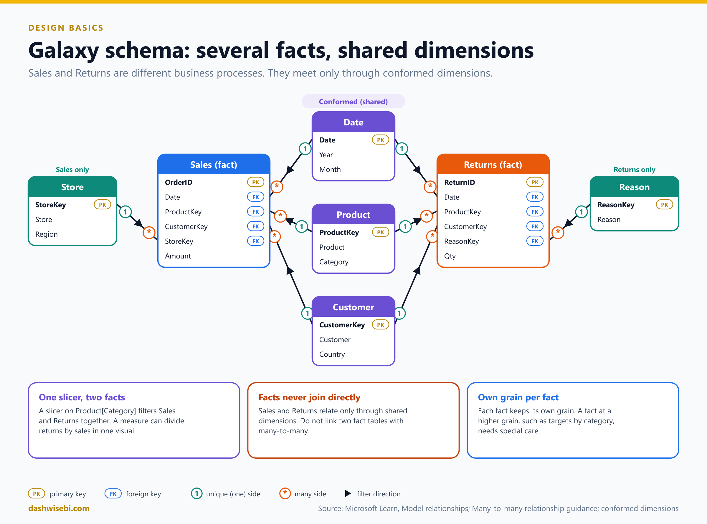
Why it works: one slicer on Product[Category] filters Sales and Returns at the same time, and a measure can divide returns by sales on one visual. Each fact table keeps its own grain.

• The facts never relate to each other directly. They meet through the shared dimensions.
• Dimensions used by only one fact table (like Store for Sales or Reason for Returns) are fine. A visual that mixes such a dimension with the other fact table will not filter it.
• If a fact table sits at a higher grain (targets by category and month), relate it at that grain, as explained in the many-to-many section.
• Learn's advice for two facts is not to link them directly with many-to-many. Add dimensions and relate each fact to them with one-to-many relationships. Then you can filter or group by any dimension column and summarize any fact column.

---

1. Configure table and column properties

Properties decide how the model looks and behaves for report authors. You set them in Model view (Properties pane), in Table view and on the Column tools tab in Report view. In Model view you can hold Ctrl and select several tables to change a property for all of them at once, for example Is hidden.

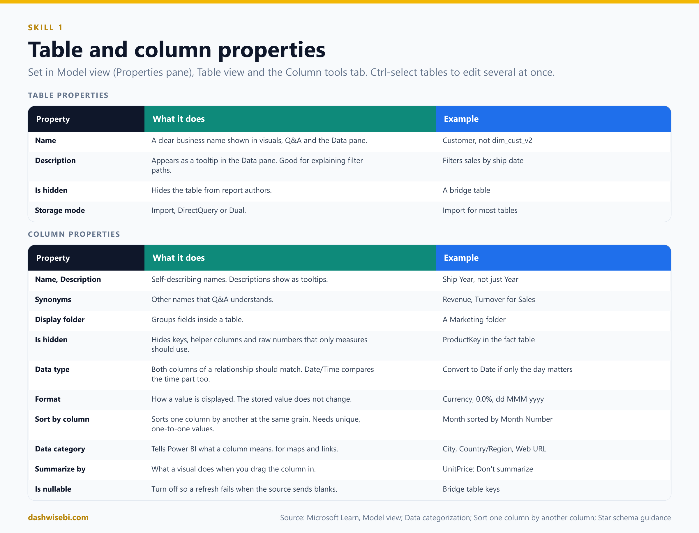
Table properties

• Name. Use clear business names, such as Customer, not dim_cust_v2. Names show up in visuals and in Q&A.
• Description. Appears as a tooltip in the Data pane when someone hovers over the table. Learn suggests using it to explain filter paths, for example "Filters reseller sales by order date".
• Is hidden. Hide tables report authors should not use directly, such as a bridge table.
• Storage mode (Import, DirectQuery, Dual), which you met in Part 1.

Column properties

• Name and Description. A column name is unique inside its table, but a bare Year in several date tables is not self-describing. Rename to Ship Year where it helps.
• Synonyms. Extra names that Q&A understands.
• Display folder. Group fields inside a table. Learn suggests display folders as a tidy alternative to extra tables, for example a Marketing folder.
• Is hidden. Hide key columns and any column report authors should not use. Typical hidden columns: ProductKey in the fact table, helper columns, and raw numeric columns that should only be used through measures.
• Data type. Both columns of a relationship should have the same type. Dates often need care: relationships on a Date/Time column compare the time part too, so convert to Date in Power Query when you only need the day.
• Format. How values are displayed: currency, percentage, decimal places, thousands separator, date pattern. It does not change the stored value.
• Sort by column. Sorts one column by another. The classic case is Month sorted by Month Number, so months run January to December instead of April, August, December. Both columns must have the same granularity, and each value must map to exactly one value of the sort column. The error "cannot use this column for sorting" means the sort column has duplicates. You set it in Report view, on the Column tools tab.
• Data category. Tells Power BI what a column means: City, Country/Region, Latitude, Longitude, Web URL, Image URL, Barcode and others. Code "CA" could be California or Canada, so setting the category lets a map visual draw the right place. Geographic categories are disabled for date or time columns.
• Summarize by (default summarization). Decides what a visual does when you drag a numeric column in: sum, average, count and so on, or none. A Unit Price column should never be summed. Set it to Don't summarize or hide it and expose measures like average or maximum price. For key columns, set Don't summarize too.
• Is nullable. If a column must never be empty, turn this off. The refresh then fails when the source delivers blanks, which catches data problems early.

Quick example

In your Date table, select Month, open Column tools > Sort by column and pick Month Number. In Sales, hide ProductKey and CustomerKey, set UnitPrice to Don't summarize, and format Line Total as currency. In Customer, set City to the City category and Country to Country/Region. These small settings are what make a model feel professional, and the exam likes them.

---

2. Implement role-playing dimensions

A role-playing dimension is one dimension that filters the same fact table in several ways. The best-known example is a date table: a sale has an order date, a ship date and a due date, and one Date table can play all three roles. Another example is an Airport table that plays departure airport and arrival airport for a flight.

In a data warehouse you simply join the same dimension several times. In Power BI there is a rule: between two tables there can only be one active relationship. Filters must follow one clear path. So you have two ways to implement a role.

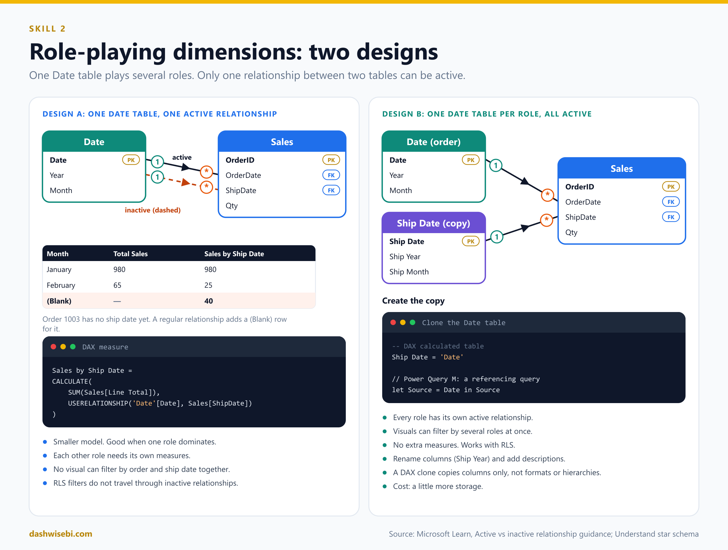
Design A: one date table, one active and the others inactive

Create a relationship from Date[Date] to Sales[OrderDate] and make it active. Create another from Date[Date] to Sales[ShipDate]. Power BI shows it as a dashed line because it is inactive. A report filter on Date flows to OrderDate. To use the ship date, a measure must turn the other relationship on for that calculation only, with USERELATIONSHIP:

Total Sales = SUM(Sales[Line Total])

Sales by Ship Date =
CALCULATE(
    [Total Sales],
    USERELATIONSHIP('Date'[Date], Sales[ShipDate])
)

Orders Shipped =
CALCULATE(
    COUNTROWS(Sales),
    USERELATIONSHIP('Date'[Date], Sales[ShipDate])
)

With the sample data, by month the two measures differ. Order 1003 has no ship date yet:

Month     | Total Sales (order date) | Sales by Ship Date
January   | 980                      | 980
February  | 65                       | 25
(Blank)   |                          | 40          <-- order 1003, not shipped yet

The (Blank) row appears because a regular relationship adds a blank virtual row for rows on the many side that have no match. Good to know, and a favorite exam detail.

Choose this design when most reports use one role, only a few measures need the others, and nobody needs to filter by order date and ship date in the same visual. It keeps the model small.

Limits of design A: you cannot plot order-date and ship-date periods side by side, every other role needs its own measures, authors who drag columns into visuals cannot use the inactive roles without measures, and row-level security filters never travel through inactive relationships, even when a measure uses USERELATIONSHIP.

Design B: one table per role, all active

Duplicate the date table once per role and give every copy its own active relationship. Learn recommends this when you need to filter by several roles at once or when you use RLS.

1. Remove any inactive relationships.
2. Optionally rename the original to describe its role, for example Order Date.
3. Create the copy. With a calculated table in DAX, or with a referencing query in Power Query.
4. Create an active relationship from the copy to the right fact column.
5. Rename columns so visuals have self-describing titles: Ship Year, Ship Month.
6. Add a table description such as "Filters sales by ship date".

-- DAX: a calculated table that clones the Date table
Ship Date = 'Date'

// Power Query M: a new query that references the Date query
let
    Source  = Date,
    Renamed = Table.RenameColumns(Source, {{"Year", "Ship Year"}, {"Month", "Ship Month"}})
in
    Renamed

A DAX clone only copies the columns. It does not copy formats, descriptions or hierarchies, so set those again. The cost of design B is a little more storage, which rarely matters because dimension tables are small.

The airport example uses the same logic. One Airport table with two relationships makes "filter by departure city and group by arrival city" impossible. Two tables, Departure Airport and Arrival Airport, each with an active relationship, solve it.

---

3. Define a relationship's cardinality and cross-filter direction

A model relationship connects one column in one table to one column in another table and passes filters along that link. Filters keep going as long as there is a path, even through several tables. When several filters reach a table, they combine with AND. Relationships do not enforce data integrity, which matters later.

How to create and edit a relationship

1. Open Model view.
2. Drag a column from one table onto a column of another table. Power BI creates the relationship and detects the settings.
3. Or choose Manage relationships and New, or double-click a relationship line, to open the dialog.
4. Check the From and To tables and columns, the Cardinality, the Cross-filter direction and the Make this relationship active box. Both columns should have the same data type.

Power BI detects the cardinality by checking which columns hold unique values. It can get this wrong when tables are not yet loaded, or when a column that should have duplicates happens to have none. You can change the setting as long as the "one" side column really holds unique values.

Cardinality

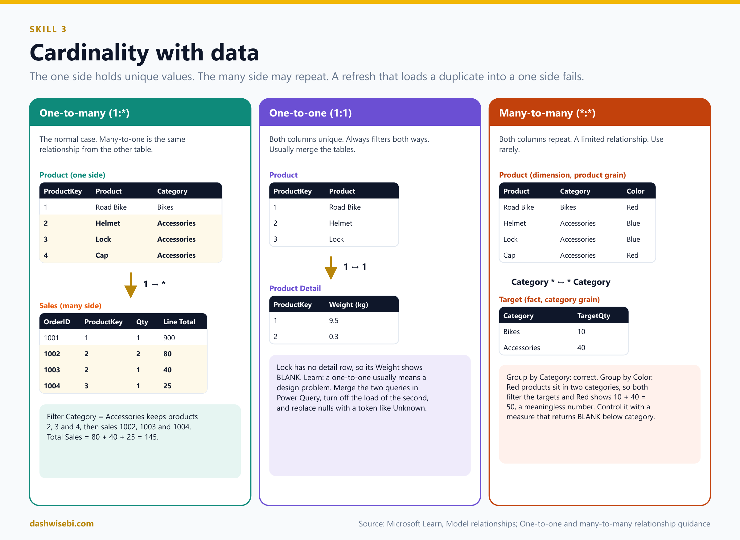
Cardinality says how rows on one side match rows on the other. The "one" side means the column contains unique values. The "many" side means it may repeat. If a refresh tries to load a duplicate into a "one" side column, the entire refresh fails.

One-to-many (1:*) and many-to-one (*:1)

This is the normal relationship, and the one you should use almost always. One-to-many and many-to-one are the same relationship. The name only follows the order of the two tables when you create it. Product to Sales is one-to-many, because Product[ProductKey] is unique. Sales to Product is many-to-one. The filter always starts on the "one" side:

Product[ProductKey] (1)  ------>  Sales[ProductKey] (*)

Filter: Product[Category] = "Accessories"
  Product rows kept:  2 Helmet, 3 Lock, 4 Cap
  Sales rows kept:    1002, 1003, 1004     (ProductKey 2, 2, 3)
  Total Sales:        80 + 40 + 25 = 145

One-to-one (1:1)

Both columns are unique. It means two tables describe the same entity, for example a Product table and a Product Detail table that both have one row per ProductKey.

Product:        ProductKey | Product        Product Detail:  ProductKey | Weight
                1          | Road Bike                       1          | 9.5
                2          | Helmet                          2          | 0.3
                3          | Lock                            (no row for key 3)

A one-to-one relationship is allowed only with both cross-filter directions. Learn says it likely points to a weak design because data is stored in two places. Products without a match show up with BLANK weights. The usual fix is to merge the two queries in Power Query into one table, turn off the load of the second, and replace nulls with a token such as "Unknown". Valid reasons for a one-to-one: a degenerate dimension taken out of a fact table, or data that truly comes from two different source groups.

Many-to-many (*:*)

Both columns may contain duplicates. We cover it in detail below, and the advice is to avoid it unless you have a specific reason.

Cross-filter direction

Cross-filter direction decides in which direction a filter travels along the relationship. The options depend on the cardinality:

Cardinality                 | Cross-filter options
One-to-many (or many-to-one)| Single, or Both
One-to-one                  | Both (always)
Many-to-many                | Single (A to B), Single (B to A), or Both

Single means the filter flows from the "one" side to the "many" side: dimension to fact. This is the default and the best choice. Both (bi-directional) means the filter also flows back from the many side to the one side. In Model view a single arrowhead shows single direction, and two arrowheads show both.

Here is a model with two dimensions and one fact. Customers and sales from our example:

Customer                              Sales (fact)
CustomerKey | Customer | Country     OrderID | ProductKey | CustomerKey | Qty
10          | Ana      | Canada      1001    | 1          | 10          | 1
20          | Ben      | Spain       1002    | 2          | 20          | 2
30          | Chen     | Japan       1003    | 2          | 10          | 1
                                     1004    | 3          | 30          | 1

A report has a Country slicer and a Product slicer. The user picks Spain.

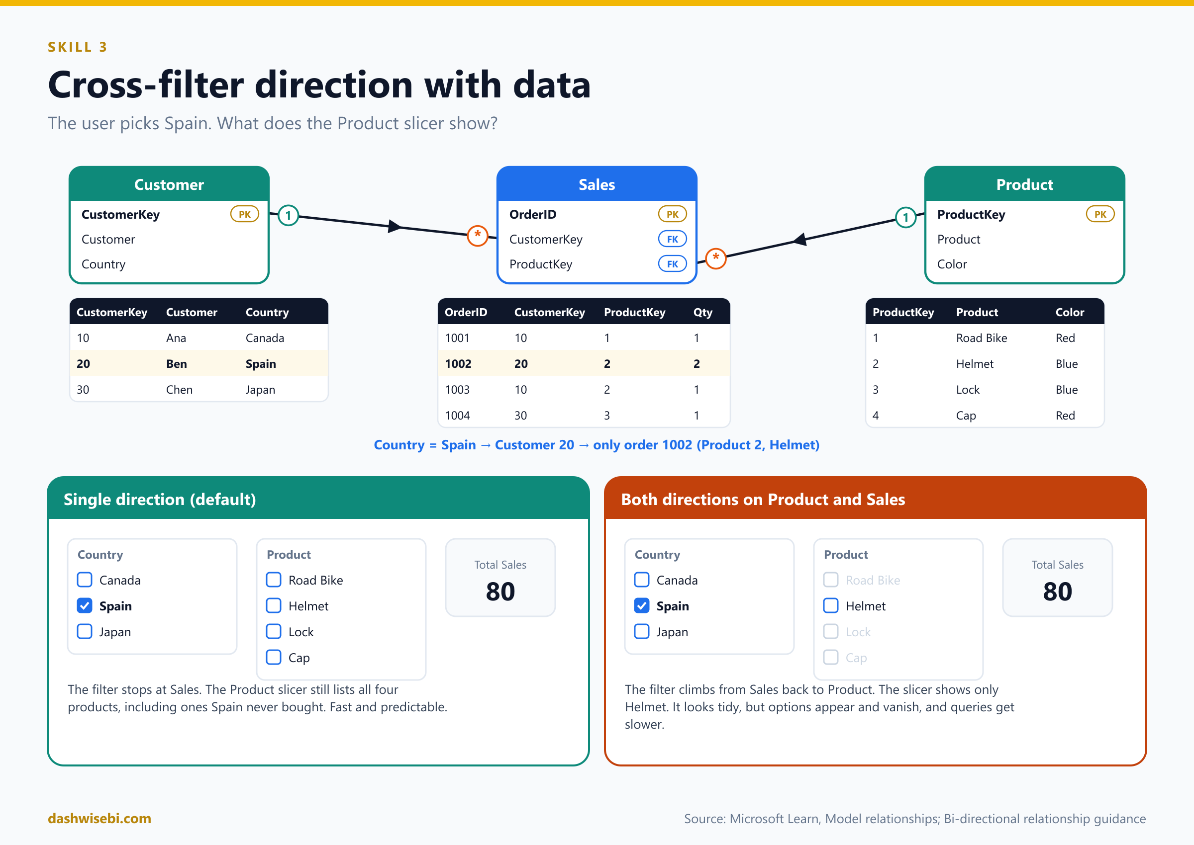
Customer[Country] = Spain
  -> Customer: Ben (20)
  -> Sales (via Customer, 1 to many): only order 1002

Single direction on Product -> Sales:
  Product slicer shows:  Road Bike, Helmet, Lock, Cap   (all four)

Both directions on Product <-> Sales:
  Sales filtered to order 1002 -> back to Product: only Helmet
  Product slicer shows:  Helmet

That second result is the "slicer options with data" behavior. It looks nice, but many report readers find it confusing when options vanish. Also, the filter had to travel uphill from fact to dimension, which costs performance.

When to use single and when to use both

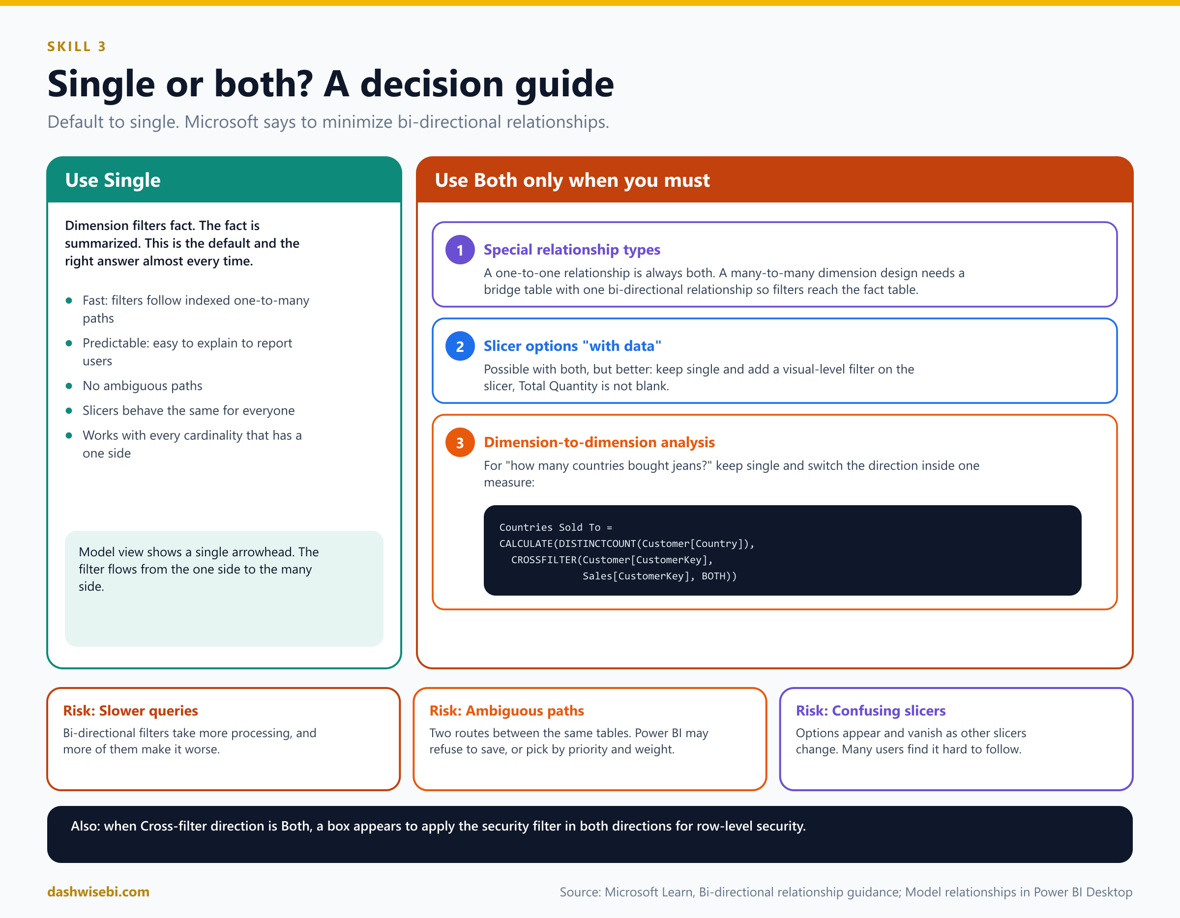
Use Single (the default) for almost everything. Dimension filters fact, fact is summarized. It is fast, predictable and easy to explain.

Microsoft says to minimize bi-directional relationships, because they can hurt query speed and confuse users. They can also create ambiguous filter paths, and Power BI may refuse to save the change. There are three scenarios where both directions solve a real problem:

1. Special relationship types. A one-to-one relationship is always both-way. A many-to-many dimension design with a bridging table needs one bi-directional relationship so filters continue across the bridge to the fact table.
2. Slicer options "with data". Possible with both, but there is a better way: keep single direction and put a visual-level filter on the product slicer, Total Quantity is not blank.
3. Dimension-to-dimension analysis (for example "how many countries bought jeans?"), where the fact table acts like a bridge. Instead of changing the relationship, switch the direction inside one measure with CROSSFILTER:

Countries Sold To =
CALCULATE(
    DISTINCTCOUNT(Customer[Country]),
    CROSSFILTER(Customer[CustomerKey], Sales[CustomerKey], BOTH)
)

Two more reasons you may enable both directions: when the option Apply security filter in both directions is needed for row-level security, and in a bridge-table design. Everywhere else, keep single. The risk list is short: slower queries, ambiguous paths, and slicers that change under the user's hands.

Active and inactive relationships

A relationship is either active (solid line) or inactive (dashed line). Only active relationships pass filters by default. An inactive one sits in the model until a calculation switches it on with USERELATIONSHIP, which you saw in the ship date example. There can be only one active path between two tables. Learn recommends active relationships whenever possible, and duplicating role-playing tables to get there. Use inactive relationships only when no visual needs two roles at once, and a few measures activate the right one.

Limited relationships

Power BI classifies every relationship as regular or limited. You do not set this. It follows from the cardinality and the data sources. A relationship is limited when there is no guaranteed "one" side, which happens when:

• the cardinality is many-to-many (even if the columns happen to be unique), or
• the relationship is cross source group, which only happens in composite models that mix storage modes or several DirectQuery sources.

In Model view a limited relationship shows parentheses ( ) after the cardinality marks. Compared with a regular one-to-many relationship inside one source:

• No index structures are built at refresh time. Tables are joined at query time, which is slower.
• No table expansion. The join uses INNER JOIN logic, so no blank virtual row is added when there is a mismatch. Unmatched rows silently disappear from results, which can hide data quality problems.
• The RELATED function cannot fetch values across a limited relationship.
• Row-level security has restrictions in some topologies.

A regular relationship, by contrast, expands tables with LEFT OUTER JOIN semantics. A sales row with a product key missing from the Product table shows up under a (Blank) product, so the mismatch stays visible. Performance order from fastest to slowest, according to Learn: one-to-many inside one source, then many-to-many through an intermediate (bridge) table with a bi-directional relationship, then many-to-many cardinality, then cross source group relationships.

Why many-to-many cardinality is not recommended

A many-to-many cardinality relationship lets you connect two columns that both contain duplicates. It looks convenient, but it brings problems:

1. It is a limited relationship, so you get the slower query-time joins, no blank row, and no RELATED.
2. It hides bad data. Unmatched rows vanish instead of appearing under (Blank).
3. The results are hard to interpret. Totals may not add up, because one row on one side matches several rows on the other (see the example below).
4. It is less flexible. If you relate two fact tables directly on an ID, you can only filter or group by that one column, not by product, date or customer.
5. It breaks the "unique key" rule. A dimension should have an ID column that is the unique "one" side of its relationships.
6. Filters can spill over: a filter on a lower-level column can match several higher-level rows, so a filter by Color may pull in whole categories (example below).

The recommended design: a bridge table

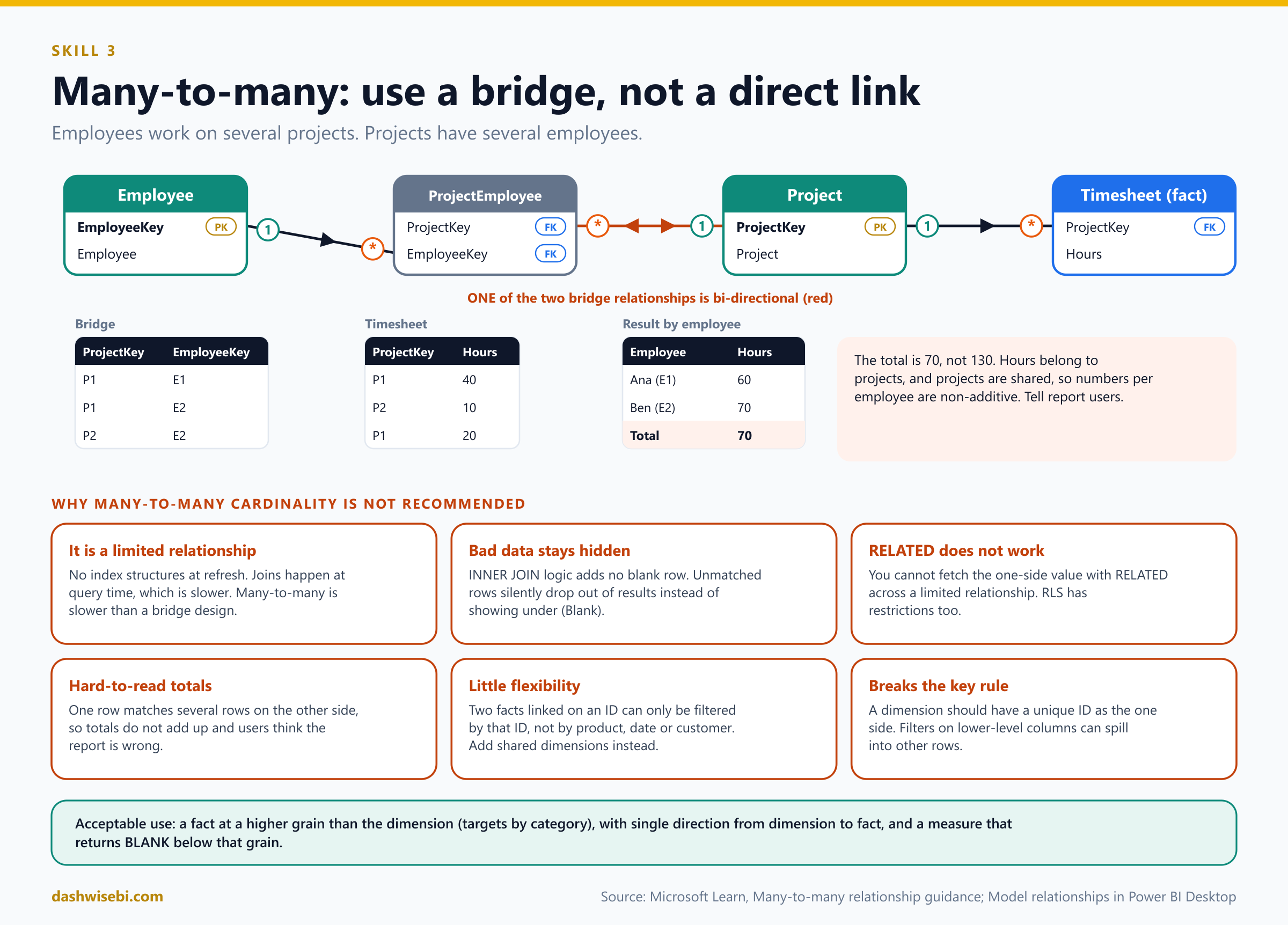
The classic many-to-many case is two dimensions. Say employees work on several projects, and each project has several employees. Add a bridging table (a factless fact table: only keys) with one row for every employee and project pair, and connect it with two one-to-many relationships. Make one of them bi-directional, so filters continue to the fact table.

Employee: EmployeeKey | Employee          Project: ProjectKey | Project
          E1          | Ana                         P1         | Website
          E2          | Ben                         P2         | Mobile app

ProjectEmployee (bridge)                  Timesheet (fact, by project)
ProjectKey | EmployeeKey                  ProjectKey | Hours
P1         | E1                           P1         | 40
P1         | E2                           P2         | 10
P2         | E2                           P1         | 20

Filter by employee Ana (E1): the bridge keeps P1, so the Timesheet shows 40 + 20 = 60 hours. Filter by Ben (E2): the bridge keeps P1 and P2, so 40 + 10 + 20 = 70 hours. The grand total over all employees is 70, not 130, because the hours belong to projects, and project hours are shared among employees. This is the trap with many-to-many: the numbers per employee are non-additive. Explain this to report users or add a note.

Guidance from Learn for this design: give each entity an ID column, create the bridge, use one-to-many relationships, set one bi-directional relationship, hide the bridge and the ID columns, and turn off Is nullable on the bridge keys. Learn also says do not relate two dimensions directly with many-to-many cardinality.

When many-to-many cardinality is acceptable: higher-grain facts

There is one case where the cardinality is useful: a fact table stored at a higher grain than the dimension. For example, sales targets are set per category, but the Product dimension is at product level. Category repeats on both sides, so there is no "one" side.

Target (fact at category grain)            Product (dimension at product grain)
Category    | TargetQty                    Product   | Category    | Color
Bikes       | 10                           Road Bike | Bikes       | Red
Accessories | 40                           Helmet    | Accessories | Blue
                                           Lock      | Accessories | Blue
                                           Cap       | Accessories | Red

Relate Product[Category] to Target[Category] with many-to-many, filtering from Product to Target in a single direction. Grouping by Category gives the right answer. Now group by Color: red products belong to two categories (Bikes and Accessories), so both categories filter the targets and the visual shows 10 + 40 = 50 for Red, which is meaningless, because targets do not exist by color. The fix is to control the summarization in a measure and return BLANK when a lower-level column filters:

Target Quantity =
IF(
    NOT ISFILTERED(Product[Product]) && NOT ISFILTERED(Product[Color]),
    SUM(Target[TargetQty])
)

Also hide the raw TargetQty column so people use only the measure. For higher-grain dates (targets by month) a one-to-many relationship works: store the first day of the period in the fact table's date column, and relate it to the date table.

Regular relationships, blanks and ambiguity

• A one-to-many regular relationship adds a blank virtual member to the "one" table when a many-side value has no match. In our example, a sales row with ProductKey = 9 appears under a (Blank) product. Fix the data instead of hiding the blank.
• Ambiguous paths. Bi-directional relationships can create two different filter routes between the same tables. Power BI picks a path by priority (for example, paths of one-to-many relationships first) and by weight, and if it still cannot decide it reports an ambiguous path error. Remove or change a relationship, or use USERELATIONSHIP.
• A table can have no relationships at all. A disconnected table (for example a what-if parameter or a slicer table) feeds measures but does not filter anything.
• A column cannot relate to another column in the same table. Parent-child hierarchies need the PATH family of DAX functions instead.

---

4. Create a common date table

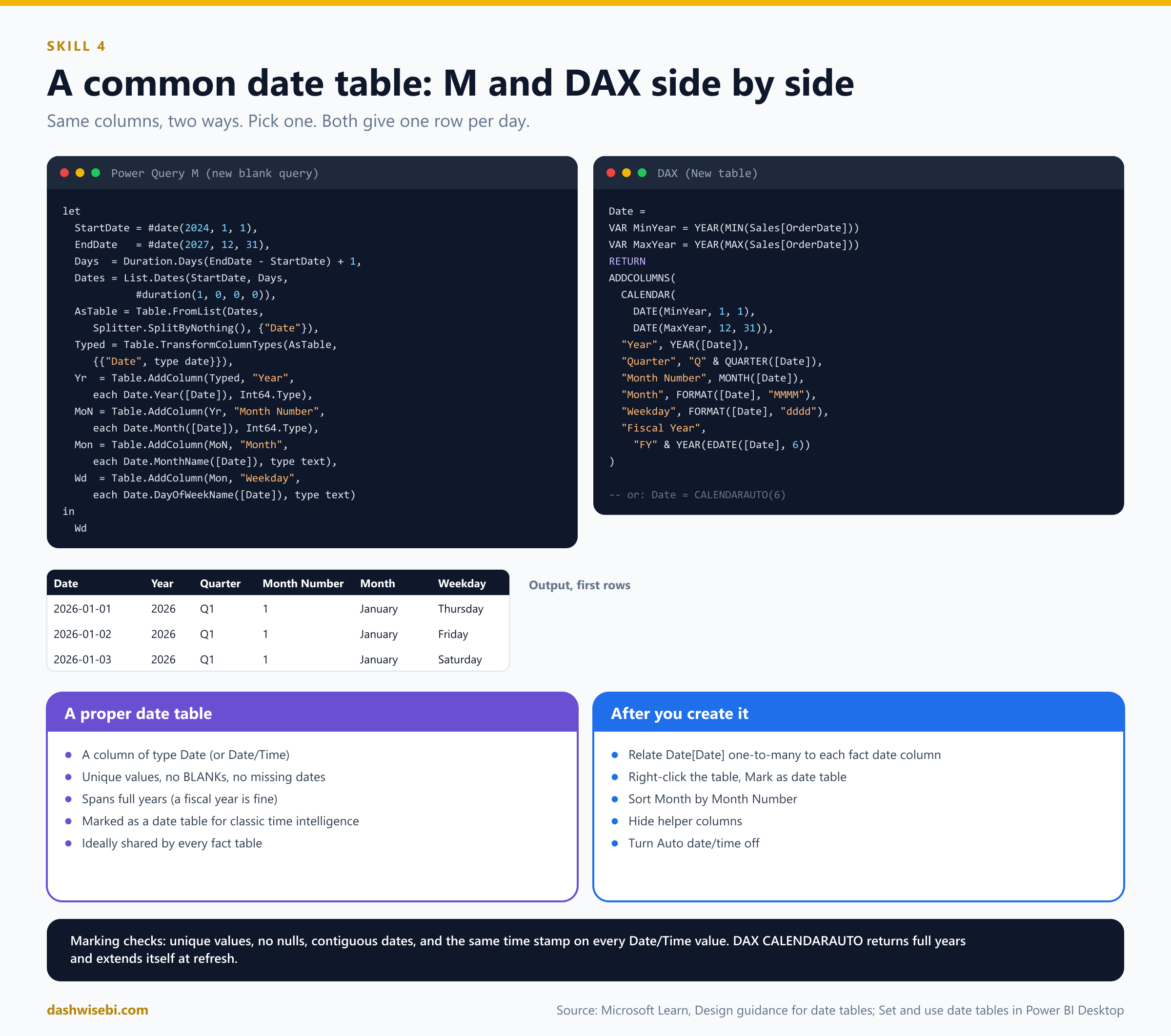
A date table is the most common table in any model. It has one row per date, and it lets people filter and group by year, quarter, month and week. DAX time intelligence functions such as TOTALYTD and SAMEPERIODLASTYEAR need one. A proper date table meets these requirements, from Learn:

• It has a column of data type Date (or Date/Time), the date column.
• The date column has unique values, no BLANKs and no missing dates.
• The dates span full years. The year does not have to be January to December: a fiscal year works too.
• For classic time intelligence, mark it as a date table.

Ways to get a date table

1. Auto date/time. Power BI builds hidden date tables for every date column. Fine for quick exploration, but you get one hidden table per date column and cannot share one table across facts.
2. Connect to an existing date dimension in a warehouse. Best, because the organization has one definition of time.
3. Generate with Power Query (M).
4. Generate with DAX (a calculated table).
5. Clone with DAX for role-playing copies.

Learn also suggests saving a fully configured date table in a Power BI template or publishing one through a dataflow, so every modeler starts from the same definition.

Power Query M: generate a date table

let
    StartDate = #date(2024, 1, 1),
    EndDate   = #date(2027, 12, 31),
    DayCount  = Duration.Days(EndDate - StartDate) + 1,
    Dates     = List.Dates(StartDate, DayCount, #duration(1, 0, 0, 0)),
    AsTable   = Table.FromList(Dates, Splitter.SplitByNothing(), {"Date"}, null, ExtraValues.Error),
    Typed     = Table.TransformColumnTypes(AsTable, {{"Date", type date}}),
    AddYear   = Table.AddColumn(Typed, "Year", each Date.Year([Date]), Int64.Type),
    AddQtr    = Table.AddColumn(AddYear, "Quarter", each "Q" & Text.From(Date.QuarterOfYear([Date])), type text),
    AddMonNo  = Table.AddColumn(AddQtr, "Month Number", each Date.Month([Date]), Int64.Type),
    AddMonth  = Table.AddColumn(AddMonNo, "Month", each Date.MonthName([Date]), type text),
    AddYM     = Table.AddColumn(AddMonth, "Year Month", each Date.ToText([Date], "yyyy-MM"), type text),
    AddWdNo   = Table.AddColumn(AddYM, "Weekday Number", each Date.DayOfWeek([Date], Day.Monday) + 1, Int64.Type),
    AddWd     = Table.AddColumn(AddWdNo, "Weekday", each Date.DayOfWeekName([Date]), type text),
    AddWknd   = Table.AddColumn(AddWd, "Is Weekend", each [Weekday Number] > 5, type logical),
    AddFY     = Table.AddColumn(AddWknd, "Fiscal Year", each "FY" & Text.From(Date.Year(Date.AddMonths([Date], 6))), type text),
    AddFM     = Table.AddColumn(AddFY, "Fiscal Month Number", each Number.Mod(Date.Month([Date]) + 5, 12) + 1, Int64.Type)
in
    AddFM

To make the range follow your data and always span full years, replace the first two steps with StartDate = Date.StartOfYear(List.Min(Sales[OrderDate])) and EndDate = Date.EndOfYear(List.Max(Sales[OrderDate])). List.Dates(start, count, step) needs a start date, how many dates, and a step of one day. The fiscal columns here assume a year that starts in July.

DAX: the equivalent calculated table

Date =
VAR MinYear = YEAR(MIN(Sales[OrderDate]))
VAR MaxYear = YEAR(MAX(Sales[OrderDate]))
RETURN
ADDCOLUMNS(
    CALENDAR(DATE(MinYear, 1, 1), DATE(MaxYear, 12, 31)),
    "Year", YEAR([Date]),
    "Quarter", "Q" & QUARTER([Date]),
    "Month Number", MONTH([Date]),
    "Month", FORMAT([Date], "MMMM"),
    "Year Month", FORMAT([Date], "yyyy-MM"),
    "Weekday Number", WEEKDAY([Date], 2),
    "Weekday", FORMAT([Date], "dddd"),
    "Is Weekend", WEEKDAY([Date], 2) > 5,
    "Fiscal Year", "FY" & YEAR(EDATE([Date], 6)),
    "Fiscal Month Number", MOD(MONTH([Date]) + 5, 12) + 1
)

• CALENDAR(start, end) returns a one-column table named Date with every day between two dates. Use it when you define the range.
• CALENDARAUTO([fiscal_year_end_month]) scans the whole model and returns full years of dates by itself. Pass the last month of your fiscal year, for example CALENDARAUTO(6) for a year that ends in June. After each refresh the table recalculates, so a new year is added automatically.
• ADDCOLUMNS adds the helper columns. You can also add each one as a separate calculated column, for example Year = YEAR('Date'[Date]).

The result, with the first rows:

Date       | Year | Quarter | Month Number | Month   | Weekday  | Is Weekend
2026-01-01 | 2026 | Q1      | 1            | January | Thursday | FALSE
2026-01-02 | 2026 | Q1      | 1            | January | Friday   | FALSE
2026-01-03 | 2026 | Q1      | 1            | January | Saturday | TRUE
2026-01-04 | 2026 | Q1      | 1            | January | Sunday   | TRUE

After you create it

1. Check the type. The Date column must be Date (not text).
2. Relate it. Create a one-to-many relationship from Date[Date] to the date column of each fact table, with single direction. If the fact table has a date key like 20260105 (an integer), relate it to a matching integer column or convert the key to Date.
3. Mark it as a date table. Right-click the table in the Fields pane, choose Mark as date table > Mark as date table, or use Table tools > Mark as date table, and pick the date column. Power BI validates that the values are unique, with no nulls and contiguous. For a Date/Time column it checks that every value has the same time stamp.
4. Sort Month by Month Number, Weekday by Weekday Number, and so on.
5. Hide the number columns.
6. Switch Auto date/time off in the report options, so Power BI does not create hidden tables next to your date table.

When you mark your own table, Power BI removes the automatic hidden date tables, and anything that used them stops working. You must mark the table when you use classic time intelligence functions, when relationships use whole-number date keys, or when you want advanced date filters in Excel PivotTables. Learn now also describes calendar-based time intelligence (preview) as the recommended approach, which does not require marking in most cases. For the exam, remember that marking is the safe answer for classic DAX time intelligence.

---

5. Identify use cases for calculated columns and calculated tables

Power BI gives you four places to compute something. Choosing the right one is the exam skill.

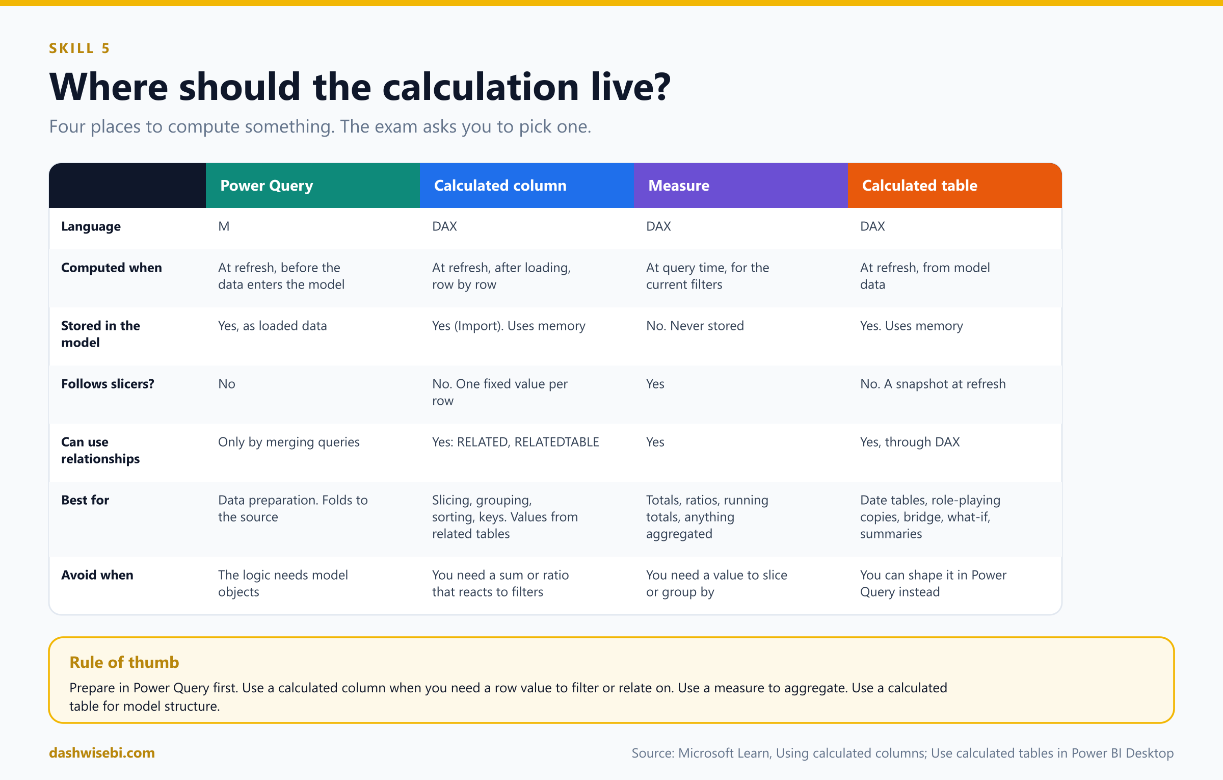
• Power Query column or query (M). Computed at refresh, before the data reaches the model. Best for data preparation and for anything that can be done at the source. It supports query folding and is the first choice for shaping data.
• Calculated column (DAX). Computed at refresh, after the data is loaded, row by row, and stored in the model (in Import mode), so it uses memory and adds refresh time. It can use other tables through relationships, for example RELATED. Best for values that you need as a column: to slice, group, sort, filter or relate on.
• Measure (DAX). Computed at query time, for the current filter context, never stored. Best for anything you aggregate: totals, ratios, running totals.
• Calculated table (DAX). Computed at refresh from a DAX expression, stored in the model. Best for date tables, role-playing copies, bridge or helper tables, and intermediate results.

Calculated columns

A calculated column has a row context: the formula runs once per row, and [Column] means "the value in this row". You create one with New column in Report, Table or Model view and type Name = expression. Unlike a Power Query custom column, a calculated column is based on data already loaded into the model, so it can mix columns from related tables.

Use a calculated column when you need to:

• slice, group or filter by a derived value, for example age band, size band or a combined label;
• sort one column by another (month name by month number);
• use the value as a relationship key, for example a combined key;
• bring a value across a relationship with RELATED or RELATEDTABLE and use it in a row-level calculation.

Do not use a calculated column for a sum, average or ratio that should react to slicers. That is a measure. A column holds one fixed value per row.

DAX and the equivalent Power Query M, for the sample Sales and Customer tables:

-- 1. Arithmetic on the same row
-- DAX (calculated column in Sales)
Line Total = Sales[Qty] * Sales[UnitPrice]
// M (custom column, in the Sales query)
Table.AddColumn(Source, "Line Total", each [Qty] * [UnitPrice], type number)

-- 2. Join text from two columns
-- DAX (Customer)
Full Name = Customer[First Name] & " " & Customer[Last Name]
// M
Table.AddColumn(Source, "Full Name", each [First Name] & " " & [Last Name], type text)

-- 3. Bands with conditions
-- DAX (Sales)
Size Band =
SWITCH(
    TRUE(),
    Sales[Qty] >= 100, "Bulk",
    Sales[Qty] >= 10,  "Standard",
    "Small"
)
// M
Table.AddColumn(Source, "Size Band",
    each if [Qty] >= 100 then "Bulk" else if [Qty] >= 10 then "Standard" else "Small", type text)

-- 4. A flag that compares two dates
-- DAX (Sales)
Shipped Late = IF(Sales[ShipDate] > Sales[DueDate], 1, 0)
// M
Table.AddColumn(Source, "Shipped Late", each if [ShipDate] > [DueDate] then 1 else 0, Int64.Type)

-- 5. A value from the other side of a relationship (many side asks the one side)
-- DAX (Sales)
Product Category = RELATED(Product[Category])
// M: merge the queries, then expand the column
Merged   = Table.NestedJoin(Sales, {"ProductKey"}, Product, {"ProductKey"}, "P", JoinKind.LeftOuter),
Expanded = Table.ExpandTableColumn(Merged, "P", {"Category"}, {"Product Category"})

-- 6. A count of related rows (one side asks the many side)
-- DAX (Customer)
Order Count = COUNTROWS(RELATEDTABLE(Sales))
// M: group the Sales query by CustomerKey, then merge the counts back (a row-by-row version is slow)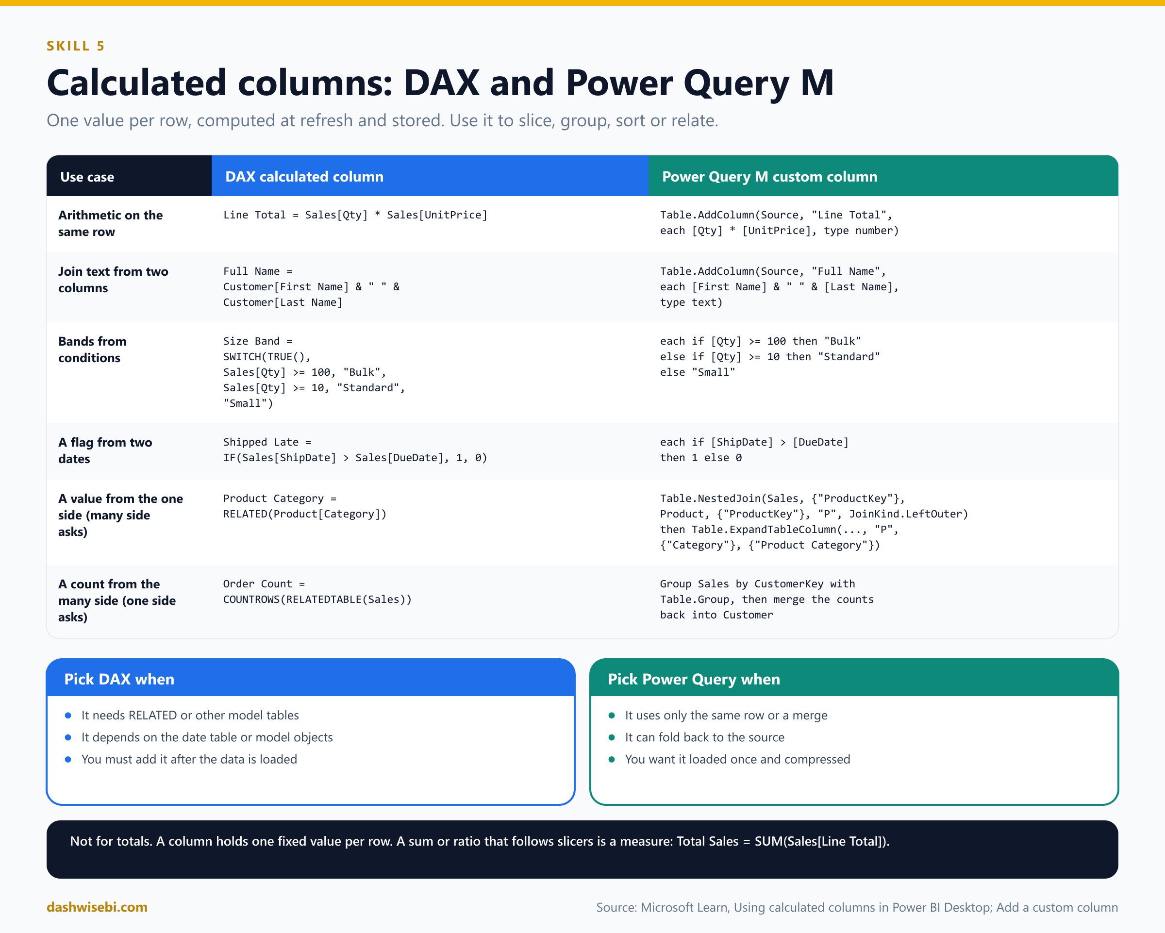

With the sample data, Line Total becomes 900, 80, 40 and 25 for the four orders, and Total Sales = SUM(Sales[Line Total]) is 1,045. Notice that Line Total is a column and Total Sales is a measure that adds it up for whatever the report filters.

How to choose between M and DAX for a column. If the logic uses only the same row, or can be merged from another query, build it in Power Query. It folds to the source when possible, loads once, and compresses well. Build it in DAX when it needs RELATED or relationship-aware logic, depends on model objects such as the date table, or must be created in the model after loading. Also remember the performance note from Learn: a materialized calculated column adds refresh time, and an unmaterialized one (DirectQuery) adds query time.

Calculated tables

A calculated table is a table made from a DAX formula that returns a table. You create one with New table in Report, Table or Model view. It is recalculated when the tables it uses are refreshed. If it uses DirectQuery data, it is not refreshed by default and only changes when the model is refreshed. Calculated tables can have relationships, measures and calculated columns like any other table, and Learn describes them as best for intermediate calculations and data you want to store as part of the model.

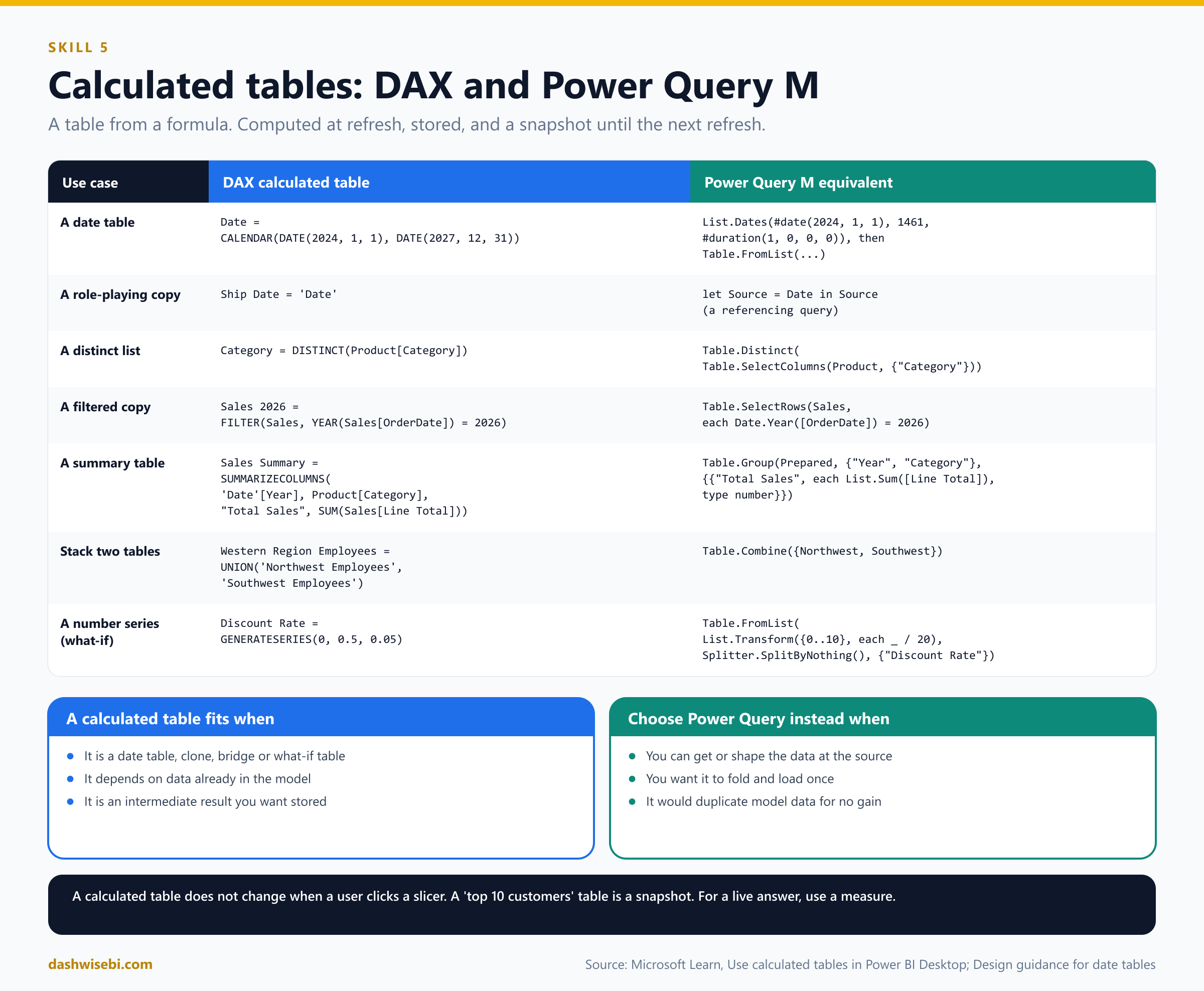
Common use cases, with DAX and the Power Query M way to get the same table:

-- 1. A date table  (see section 4)
Date = CALENDAR(DATE(2024, 1, 1), DATE(2027, 12, 31))
// M: List.Dates + Table.FromList (see section 4)

-- 2. A role-playing copy of a dimension
Ship Date = 'Date'
// M: a new query that references the Date query (Source = Date)

-- 3. A distinct list: build a dimension from a column
Category = DISTINCT(Product[Category])
// M
let Source = Table.Distinct(Table.SelectColumns(Product, {"Category"})) in Source

-- 4. A filtered copy of a table
Sales 2026 = FILTER(Sales, YEAR(Sales[OrderDate]) = 2026)
// M
Table.SelectRows(Sales, each Date.Year([OrderDate]) = 2026)

-- 5. A summary table at a higher grain (an aggregate for speed)
Sales Summary =
SUMMARIZECOLUMNS(
    'Date'[Year],
    Product[Category],
    "Total Sales", SUM(Sales[Line Total])
)
// M
Table.Group(SalesWithCategory, {"Year", "Category"}, {{"Total Sales", each List.Sum([Line Total]), type number}})

-- 6. Stack two tables with the same columns
Western Region Employees = UNION('Northwest Employees', 'Southwest Employees')
// M
Table.Combine({#"Northwest Employees", #"Southwest Employees"})

-- 7. A number series for a what-if parameter (a disconnected table)
Discount Rate = GENERATESERIES(0, 0.5, 0.05)
// M
Table.FromList(List.Transform({0..10}, each _ / 20), Splitter.SplitByNothing(), {"Discount Rate"})

When is a calculated table the right answer, and when is it not?

• Right: the date table when you want CALENDARAUTO's automatic range, a quick role-playing clone, a bridge table built from existing columns, a disconnected slicer or what-if table, or an intermediate table that depends on other model data.
• Wrong: data that you can get from the source, or shape in Power Query. M queries fold, load once, and do not add DAX work at refresh. A calculated table does not make a table "from nothing", it makes it from data already in the model, which duplicates storage.
• A calculated table is a snapshot at refresh. A "top 10 customers" calculated table does not change when a user clicks a slicer. For that you need a measure.
• Keep an eye on model size. Every calculated table and calculated column uses memory.

Both calculated columns and calculated tables are also affected by the storage mode. In an Import model they are computed at refresh. Support in Direct Lake models is limited today (preview, only for the user-context type), so check the storage mode before you promise a design.

---

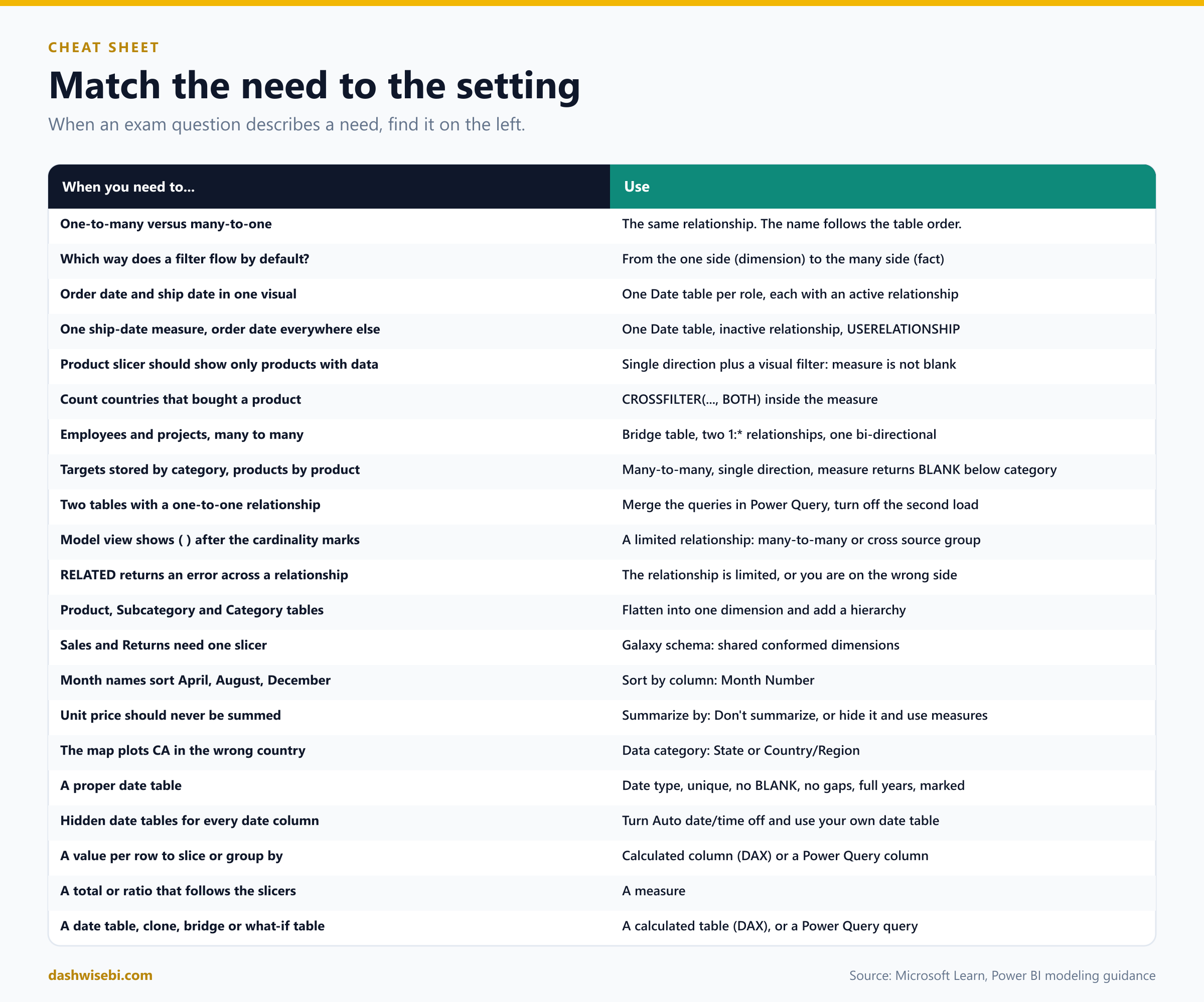
Cheat sheet

Common mix-ups

• "One-to-many and many-to-one are different relationships." They are the same. The name follows the order of the tables.
• "Filters flow from the many side to the one side." By default they flow from the one side (dimension) to the many side (fact).
• "Both directions make the model more accurate." They make it slower and can make paths ambiguous. Use single by default.
• "A one-to-one relationship can be single direction." It is always both.
• "A table property marks a table as fact or dimension." The relationship cardinality decides it.
• "I can have as many active relationships between two tables as I like." Only one is active. The others are inactive (dashed).
• "USERELATIONSHIP changes the relationship permanently." It switches one on only inside that calculation.
• "RLS works through inactive relationships." RLS filters do not travel through them.
• "Many-to-many cardinality is the easy way to relate two dimensions." Use a bridge table with two one-to-many relationships instead.
• "Limited relationships are a setting." They follow from many-to-many cardinality or cross-source-group relationships. You cannot switch them on.
• "A DAX clone of the Date table copies my formats and hierarchies." It only copies columns.
• "A date table can have gaps if I filter later." A date table needs every date and full years.
• "Sort by column can use any column." The sort column must have one value per value of the sorted column, with the same granularity.
• "A calculated column is just a measure for each row." It is stored, computed at refresh, and does not react to slicers. Totals that follow filters belong in measures.
• "Calculated tables update when a slicer changes." They recalculate at refresh.
• "Snowflakes are better because they are normalized." For Power BI, flatten dimensions into one table unless you have a clear reason.

Try it yourself: eight exam-style questions

Cover the answers and test yourself.

Question 1

A Sales table has OrderDate and ShipDate. A report must show a chart of sales by order month next to a chart of sales by ship month. What do you do?

Answer: Create a second date table for the ship date (a DAX clone such as Ship Date = 'Date' or a referencing query) and give each date table its own active relationship. One date table with an inactive relationship cannot filter both roles at the same time.

Question 2

Only one measure, Orders Shipped, needs the ship date. All other measures use the order date, and no visual needs both. What is the simplest design?

Answer: One date table with an active relationship to OrderDate and an inactive one to ShipDate, and the measure uses CALCULATE(COUNTROWS(Sales), USERELATIONSHIP('Date'[Date], Sales[ShipDate])).

Question 3

You create a relationship from Product[Category] to Target[Category]. Both columns contain duplicates. Which cardinality does Power BI offer, and what should you watch for?

Answer: Many-to-many, because Target is at a higher grain than Product. It is a limited relationship. Control summarization with a measure that returns BLANK when columns below category (product, color) are filtered, and hide the raw target column.

Question 4

Employees work on several projects and projects have several employees. How do you model it?

Answer: Add a bridge table of employee and project keys, create one-to-many relationships from Employee and from Project to the bridge, and set one of them to filter in both directions. Hide the bridge. Do not relate the two dimensions directly with many-to-many.

Question 5

A product slicer should only show products that were sold to the selected country. A colleague wants to switch the Product to Sales relationship to Both. Is there a better way?

Answer: Yes. Keep the relationship single and add a visual-level filter to the product slicer: Total Quantity is not blank. Bi-directional filters cost performance and confuse users.

Question 6

You mark Date as a date table and get an error. Which three checks does Power BI make on the date column?

Answer: The values must be unique, contain no nulls, and be contiguous (no missing dates). A Date/Time column must also have the same time stamp on every value.

Question 7

The month names in a chart sort April, August, December. How do you fix it?

Answer: Add a Month Number column at the same granularity and set Month to Sort by column Month Number. Each month name must map to exactly one number.

Question 8

You need a column on Sales that shows the product category from the Product table, for slicing. Which DAX do you use, and what is the Power Query alternative?

Answer: A calculated column Product Category = RELATED(Product[Category]). The alternative is to merge Sales with Product in Power Query and expand the Category column. In a star schema you rarely need either: slice by Product[Category] directly, because the relationship already filters Sales.

Where to go next

Practise on a small model of your own. Draw the star schema first, then create the relationships, break one on purpose, and watch what the numbers do. That is the fastest way to remember it.

• Try our free practice quizzes
• Join the Data Days study group
• Read Episode 2: Transform and load data in Power Query
• Read Part 1: Getting, connecting and profiling data

Microsoft Learn references

• PL-300 study guide
• Understand star schema and the importance for Power BI
• Model relationships in Power BI Desktop
• Active vs inactive relationship guidance
• Bi-directional relationship guidance
• Many-to-many relationship guidance
• One-to-one relationship guidance
• Design guidance for date tables in Power BI Desktop and Set and use date tables
• Using calculated columns in Power BI Desktop and Use calculated tables in Power BI Desktop
• Use Model view in Power BI Desktop, Data categorization and Sort one column by another column
• CALENDAR, CALENDARAUTO, USERELATIONSHIP and CROSSFILTER
• Modeling dimension tables in Warehouse for conformed dimensions and role-playing dimensions

See you in the next episode, where we move on to model calculations with DAX.