PL-300 Episode 4: Advanced DAX & Model Performance

PowerBI consultant ·
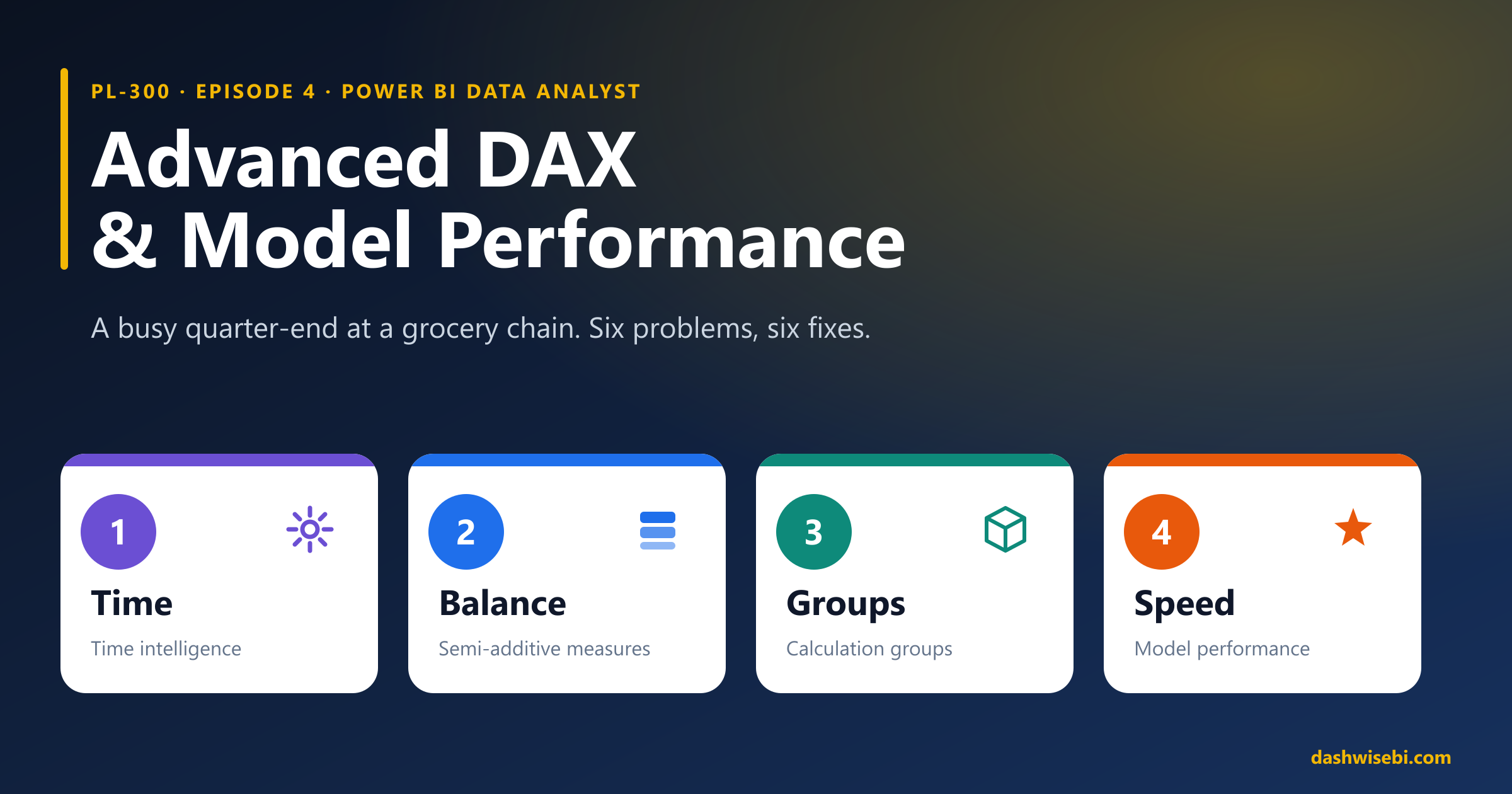
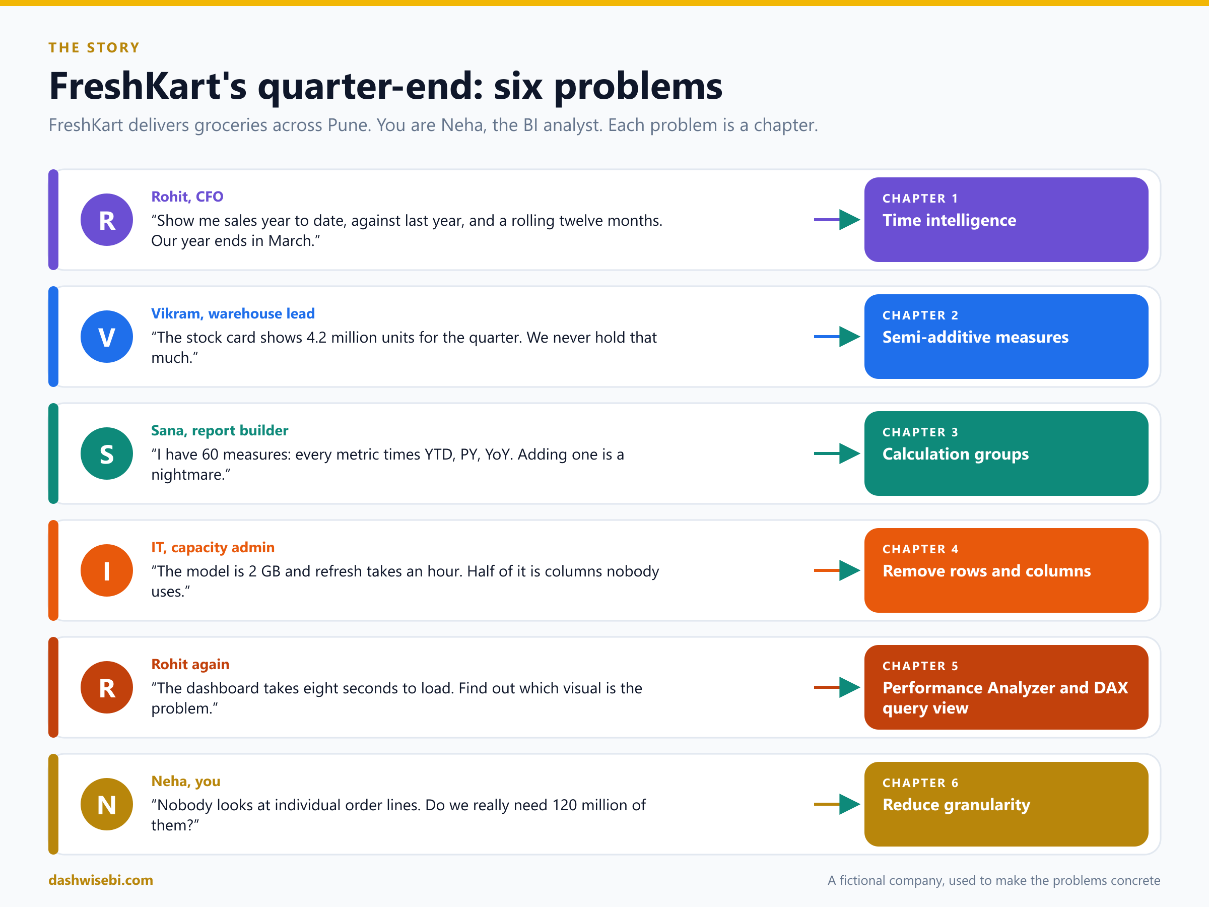
It is the last week of the quarter at FreshKart, a grocery delivery company in Pune. The finance floor smells of chai and panic. You are Neha, the BI analyst, and six people are queuing at your desk.
Welcome to Episode 4 of our PL-300 series. In Episode 3 you built a sound data model: a star schema, the right relationships and a date table. Now the model has to answer harder questions, and answer them fast. These are the topics for this episode:
- Implement time intelligence measures
- Create semi-additive measures
- Create calculation groups
- Improve performance by identifying and removing unnecessary rows and columns
- Identify poorly performing measures, relationships, and visuals by using Performance Analyzer and DAX query view
- Improve performance by reducing granularity
Like the latest DP-700 episodes, this post is a working day instead of a reference list. Every chapter has the same rhythm:
- The problem. Someone brings you a request.
- Pause and decide. Try the choice first. The answer is hidden behind a click.
- Why. The reasoning, the DAX and the diagrams.
- Exam lens. What PL-300 tends to ask, and the traps.
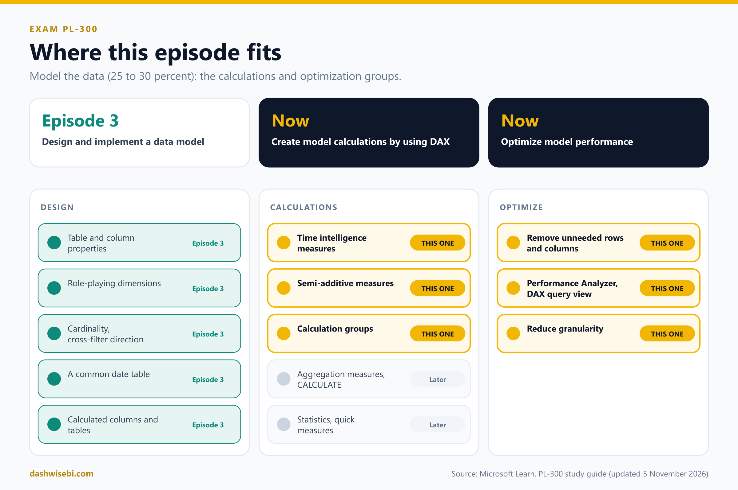
A note on wording. The study guide Microsoft updated on 5 November 2026 lists these topics under Create model calculations by using DAX and Optimize model performance. Calculation groups are in your session outline, so they are in this post. The other topics of the DAX group (single aggregation measures, CALCULATE filters, basic statistical functions and quick measures) are not covered here. Because every chapter leans on CALCULATE, a one-minute refresher follows.
The FreshKart model
Everything in this post uses one small model, the star schema from Episode 3:
- Sales (fact): one row per order line, with
OrderDate,ProductKey,StoreKey,Qty,NetAmountandCost. - Inventory (fact): one row per product, per store, per day, with
StockUnits. A daily photo of the shelves. - Date, Product, Store, Customer (dimensions). The Date table is a proper date table, one row per day, related to
Sales[OrderDate]andInventory[SnapshotDate].
CALCULATE in one minute. CALCULATE ( <expression>, <filter>, ... ) evaluates the expression in a changed filter context. A filter can be a column condition, or a table of dates. Time intelligence functions such as SAMEPERIODLASTYEAR return exactly that: a table of dates, which CALCULATE uses as a filter on the Date table. Keep this in mind. It explains almost everything in Chapters 1 and 2.
Chapter 1. Rohit asks: this year, last year, and the trend
Rohit, the CFO, drops a printout on your desk. Three lines are circled in red.
Rohit: Sales year to date. Against the same period last year. And a rolling twelve months, so I can see the trend without the seasons. Oh, and our year ends in March.
Three requests, and time intelligence is the tool. Before the explanation, try three small decisions.
Pause and decide. FreshKart's financial year ends on 31 March. What do you add to TOTALYTD so that “year to date” starts on 1 April?
The optional year_end_date argument: TOTALYTD ( [Sales], 'Date'[Date], "3/31" ). It is a text literal. The year part is ignored, and Microsoft recommends the month/day form so the string always resolves to a date.
Pause and decide. A colleague passes Sales[OrderDate] (the date column in the fact table) to SAMEPERIODLASTYEAR. The stores are closed on a few festival days, so there are no sales rows for them. The measure errors. Why, and what is the fix?
Classic time intelligence needs a complete date column: if there are missing dates between the first and last date, an error is thrown. A fact-table date column has gaps. The fix is a dedicated date table with one row for every day, and using its Date column in every time intelligence function. (Calendar-based time intelligence, in preview, operates on sparse dates as they are.)
Pause and decide. It is 14 November. Rohit compares Sales YTD this year (six weeks of the new financial year) with Sales for the whole of last year. Is that a fair comparison?
No. It compares a partial year with a full year. Compare like with like: this year's YTD against last year's YTD, with CALCULATE ( [Sales YTD], SAMEPERIODLASTYEAR ( 'Date'[Date] ) ).
Why: the date table comes first
Time intelligence functions work on a date table. Microsoft's guidance is blunt: before using any of them, mark one of the tables that contains a date column as the Date Table. Episode 3 showed how to build one. Remember three rules for the classic functions:
- Use a column from the date table, never the date in the fact table.
- The dates must be contiguous: no gaps between the first and last date.
- One date table, related to every fact table that needs time analysis.
Why: the measures
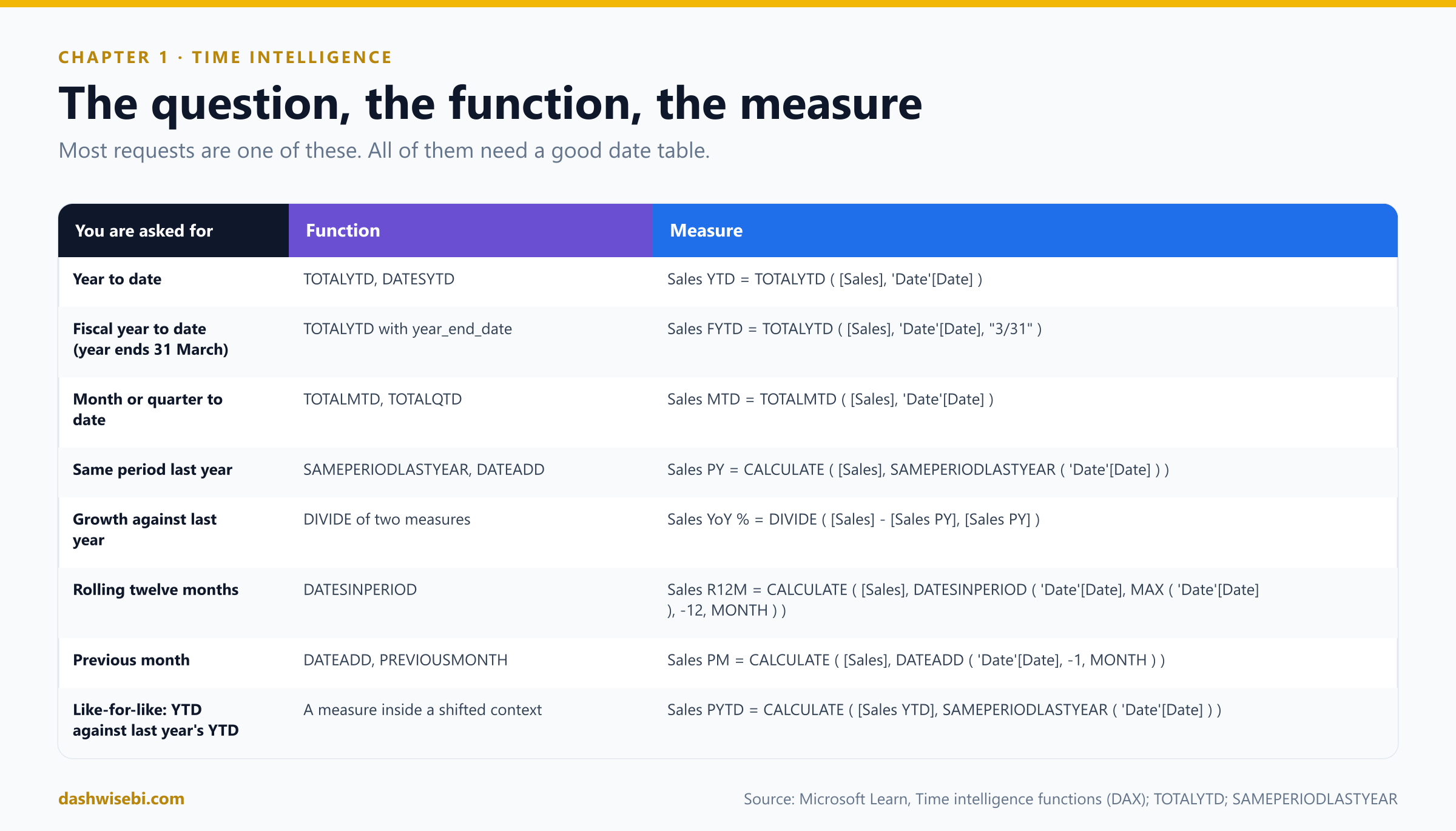
Sales = SUM ( Sales[NetAmount] )

Sales YTD  = TOTALYTD ( [Sales], 'Date'[Date] )
Sales FYTD = TOTALYTD ( [Sales], 'Date'[Date], "3/31" )     -- year ends 31 March
Sales MTD  = TOTALMTD ( [Sales], 'Date'[Date] )

Sales PY   = CALCULATE ( [Sales], SAMEPERIODLASTYEAR ( 'Date'[Date] ) )
Sales YoY % = DIVIDE ( [Sales] - [Sales PY], [Sales PY] )

Sales R12M =
CALCULATE (
    [Sales],
    DATESINPERIOD ( 'Date'[Date], MAX ( 'Date'[Date] ), -12, MONTH )
)

Sales PYTD = CALCULATE ( [Sales YTD], SAMEPERIODLASTYEAR ( 'Date'[Date] ) )TOTALYTDis a shortcut: it evaluates the expression for the year to date in the current context.TOTALMTDandTOTALQTDwork the same way for months and quarters. The optional filter andyear_end_datearguments come after the date column.SAMEPERIODLASTYEARreturns the dates of the current context shifted one year back. It gives the same dates asDATEADD ( dates, -1, YEAR ). UseDATEADDwhen you want another step: its interval can be year, quarter, month or day (and week, for calendar-based use).DIVIDEhandles the divide-by-zero case, so a year with no prior sales shows blank instead of an error.DATESINPERIODbuilds a window: starting from the last visible date (MAX), go back 12 months. In a visual by month, each month shows the twelve months ending in it.- A measure inside a shifted context (
Sales PYTD) is a powerful pattern: buildSales YTDonce, then askCALCULATEto evaluate it a year earlier. - If the context is not a contiguous set of dates (for example a non-adjacent multi-selection),
DATEADDreturns an error. Slice time with a proper date hierarchy.
Three ways to do time
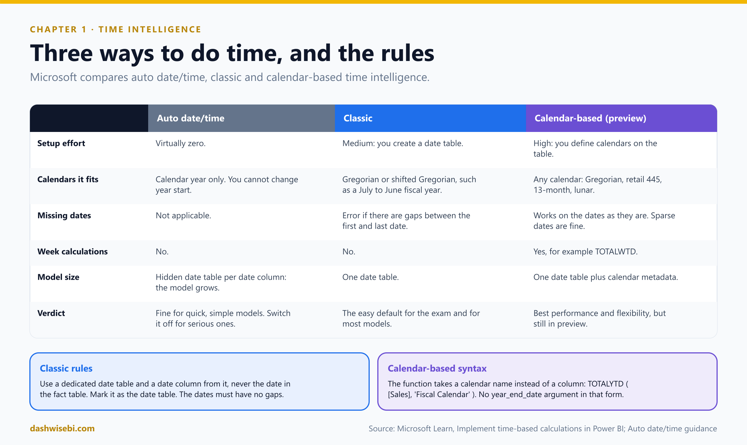
Microsoft compares three tools for time-based calculations. Auto date/time needs no setup but creates a hidden date table for every date column, which grows the model. Classic time intelligence needs a date table, assumes a Gregorian or shifted Gregorian calendar, and fails on gaps. Calendar-based time intelligence is the newest option and is still in preview:
- A calendar is metadata on a table that says which columns mean which unit of time (Year, Quarter, Month, Week, Date and so on). Turn it on with the Enhanced DAX Time Intelligence preview feature, then use Calendar options on the table.
- You then pass the calendar instead of a column:
TOTALYTD ( [Sales], 'Fiscal Calendar' ). There is noyear_end_datein this form, because the calendar already knows when the year ends. - It supports any calendar (retail 445, 13-month, lunar), sparse dates, week-based functions such as
TOTALWTD, and can be faster. - Limits: you cannot author calendars in the Power BI service yet, cannot use them with live-connected or composite models, should not mix them with auto date/time tables, and cannot nest calendar-based functions.
One more warning from the documentation: avoid homemade tricks that add offset columns to the date table (for example a “last year” column). The DAX looks simple, but the columns inflate the model and slow refresh as it grows.
Rohit reads the three numbers, nods once, and says the most dangerous sentence in finance: “Good. Now, the inventory report.”
Exam lens
- Time intelligence needs a date table, marked as such, with no gaps.
- Fiscal year end: the
year_end_dateargument, as month/day text. - Same period last year:
CALCULATEwithSAMEPERIODLASTYEAR(orDATEADD). - Rolling window:
DATESINPERIOD. - Auto date/time is fine for simple models, but it grows the model.
Chapter 2. Vikram asks: how much stock do we hold?
Vikram, the warehouse lead, holds his phone up like evidence.
Vikram: The stock card says 4.2 million units for the quarter. FreshKart has never held 4.2 million units of anything. It is a number from a parallel universe.
You already know why. The Inventory table has a row per product, per store, per day, and the card adds up 90 days of photos. Here is a miniature of the problem:
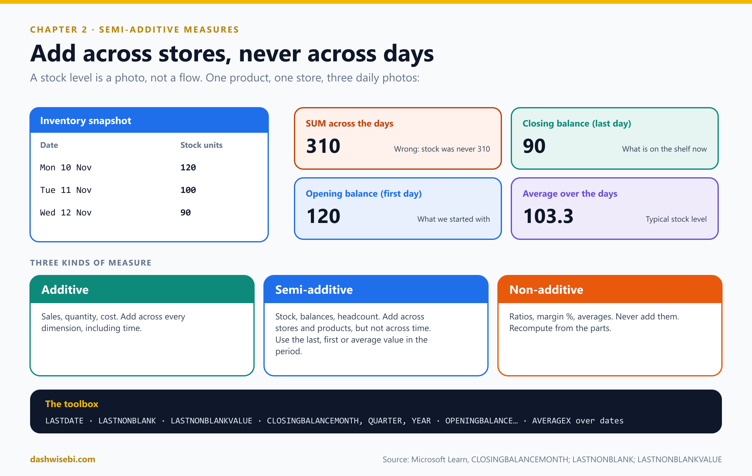
Pause and decide. Which of these is additive, which is semi-additive and which is non-additive: (a) revenue, (b) stock on hand, (c) gross margin percentage?
(a) Additive: add it across every dimension, including time. (b) Semi-additive: add it across products and stores, but across time take the last (or first, or average) value. (c) Non-additive: never add a ratio. Recompute it from its parts.
Pause and decide. Vikram wants the stock at the end of each month. Which function family gives you that directly?
CLOSINGBALANCEMONTH (and its QUARTER and YEAR relatives). It evaluates the expression at the last date of the month in the current context. The Microsoft example computes a month-end inventory value from the product inventory table.
Pause and decide. Stock is photographed every day except Sundays, when the store is closed. Your “stock on the last day” measure shows blank for any month that ends on a Sunday. What do you use instead of LASTDATE?
LASTNONBLANK (or LASTNONBLANKVALUE). It returns the last date for which the expression is not blank, so a Sunday with no photo falls back to the Saturday before it.
Why: the patterns
-- Stock on the last day of the period (a closing balance)
Stock Closing =
CALCULATE ( SUM ( Inventory[StockUnits] ), LASTDATE ( 'Date'[Date] ) )

-- The built-in closing balance for month ends
Stock Month End =
CLOSINGBALANCEMONTH ( SUM ( Inventory[StockUnits] ), 'Date'[Date] )

-- Safe when the last day has no photo: use the last date that has data
Stock Last Known =
CALCULATE (
    SUM ( Inventory[StockUnits] ),
    LASTNONBLANK ( 'Date'[Date], CALCULATE ( SUM ( Inventory[StockUnits] ) ) )
)

-- The same, in one function
Stock Last Known 2 =
LASTNONBLANKVALUE ( 'Date'[Date], SUM ( Inventory[StockUnits] ) )

-- The first day (an opening balance)
Stock Opening =
CALCULATE ( SUM ( Inventory[StockUnits] ), FIRSTDATE ( 'Date'[Date] ) )

-- Typical stock over the period: average of the daily totals
Stock Average =
AVERAGEX ( VALUES ( 'Date'[Date] ), CALCULATE ( SUM ( Inventory[StockUnits] ) ) )LASTDATEreturns the last date in the current context as a one-row table. As aCALCULATEfilter, it moves the evaluation to that single day. The sum then adds across stores and products on that day, which is exactly what a semi-additive measure should do.CLOSINGBALANCEMONTHtakes an expression and a date column (or, in the preview, a calendar). TheOPENINGBALANCEfamily does the same for the first date, and there are week, quarter and year versions.LASTNONBLANK ( column, expression )returns a table with one row: the last value of the column for which the expression is not blank.LASTNONBLANKVALUEgoes further and returns the value of the expression at that date. Microsoft notes the difference: inLASTNONBLANKVALUEthe column is added to the filter context while the expression is evaluated.- A caution: “last non-blank date” is found across the whole current selection. If one store stopped reporting earlier than the others, it contributes nothing on the last date. Check this case in your data.
AVERAGEXover the dates gives a typical level, when “the average stock this month” is the real question.- The Learn pages mark these time functions as discouraged in visual calculations, because they are likely to return meaningless results there. Write them as measures.
The stock card now shows 41,800 units. Vikram squints at it, then nods. “That is a warehouse I recognize.”
Exam lens
- Balances, stock and headcount are semi-additive: sum across everything except time.
- The usual answers:
LASTDATEorCLOSINGBALANCEMONTHfor the period end,FIRSTDATEorOPENINGBALANCEfor the start,LASTNONBLANKwhen the last day can be empty, andAVERAGEXfor a typical level. - Summing a snapshot across days is the classic wrong answer.
Chapter 3. Sana asks: please make it stop
Sana, the report builder, shares her screen. The measures list scrolls for a long time.
Sana: Sales, Sales YTD, Sales PY, Sales YoY, Sales YoY %. Then the same five for Cost. And Margin, Orders, Units, Basket. That is thirty measures, and Rohit just asked for a sixth metric. I will have to write five more. And fix the one I got wrong in March.
This is the textbook problem calculation groups solve. Think of a calculation group as a set of reusable time views that wrap any measure.
Pause and decide. Sana has a column Sales[NetAmount] that she drags straight into a matrix and aggregates with Sum (an implicit measure). Will a calculation item such as YTD apply to it?
No. Calculation items apply only to explicit measures (ones you create with New measure). That is why Power BI asks you to turn on Discourage implicit measures when you add a calculation group. It then hides the sum symbol on columns and stops you dropping them into visuals as values. Implicit measures already in visuals continue to work.
Pause and decide. The YoY % item returns 0.12, shown as $0.12 because the underlying measure is a currency. What do you set on the calculation item?
A dynamic format string. Calculation items use the underlying measure's format by default. Select the item, turn on Dynamic format string in the properties, and give it a DAX expression that returns the format, such as one that produces #,##0.00%.
Pause and decide. The model has two calculation groups: Time Calculation and Currency. A visual uses [Sales] with items from both. Which setting decides which one applies first?
The precedence property of each calculation group, in the properties pane.
Why: how a calculation group works
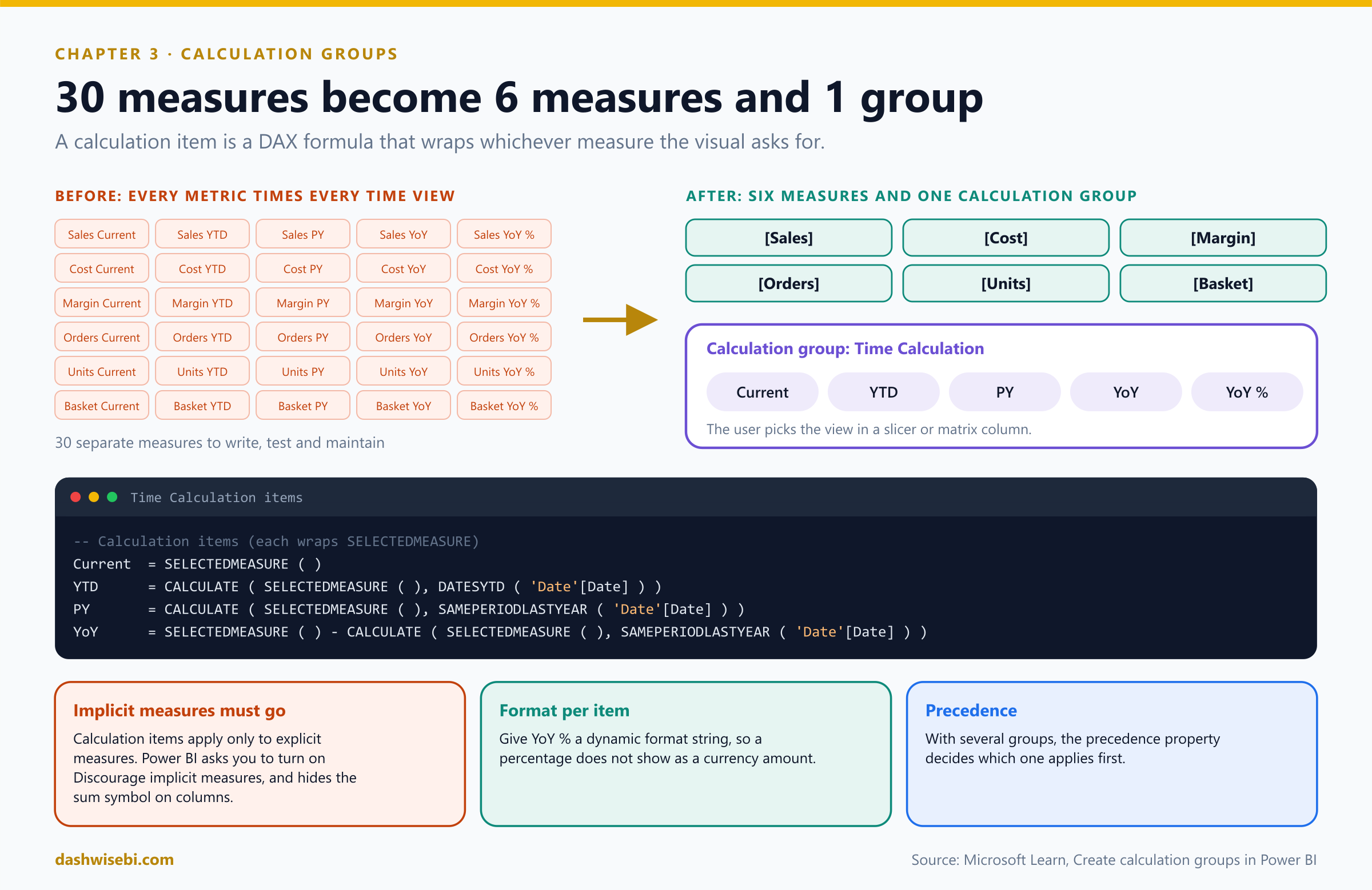
A calculation group is a special table. Its main column lists the calculation items: each row is one item: a DAX expression that is applied to the measure in the visual. The placeholder for “the measure the visual asked for” is SELECTEDMEASURE ( ).
Build it in Power BI Desktop
- Open Model view, and select Calculation group in the ribbon.
- If Discourage implicit measures is off, accept the prompt. A group appears with a first item,
SELECTEDMEASURE ( ). - Rename the group (for example Time Intelligence), the group's column (Time Calculation) and the first item (Current).
- Add more items with New calculation item and type the DAX in the formula bar. Reorder them in the properties pane.
- Optionally set a dynamic format string on an item, and a precedence on the group.
The items for FreshKart:
Current = SELECTEDMEASURE ()

YTD = CALCULATE ( SELECTEDMEASURE (), DATESYTD ( 'Date'[Date] ) )

PY = CALCULATE ( SELECTEDMEASURE (), SAMEPERIODLASTYEAR ( 'Date'[Date] ) )

YoY =
SELECTEDMEASURE ()
    - CALCULATE ( SELECTEDMEASURE (), SAMEPERIODLASTYEAR ( 'Date'[Date] ) )

YoY % =
DIVIDE (
    SELECTEDMEASURE ()
        - CALCULATE ( SELECTEDMEASURE (), SAMEPERIODLASTYEAR ( 'Date'[Date] ) ),
    CALCULATE ( SELECTEDMEASURE (), SAMEPERIODLASTYEAR ( 'Date'[Date] ) )
)
Then use the group in a report. In a matrix, put Month on rows, the Time Calculation column on columns and a measure such as [Orders] in values: you get that measure once for every item. Put the same column in a slicer, and one chosen item applies to every measure on the page. You can also call an item from a measure:
Sales YoY % (from the group) =
CALCULATE ( [Sales], 'Time Intelligence'[Time Calculation] = "YoY %" )
Things that bite
- Measures become variant. As soon as a calculation group exists, Power BI reports use the variant data type for all measures. If you remove all groups, the measures return to their original types. A variant measure can make a dynamic format string that re-uses a measure show an error. Wrap it:
FORMAT ( [Dynamic format string], "" ). - Text measures break math items. A measure that returns text (for a dynamic title, say) gives “Cannot convert value of type Text to type Numeric” when an item does arithmetic on it. Guard the item with
ISNUMERIC:
Calculation item safe =
IF (
    ISNUMERIC ( SELECTEDMEASURE () ),
    SELECTEDMEASURE () * 2,
    SELECTEDMEASURE ()          -- leave non-numeric measures alone
)- Some measures should be left alone. A year-to-date of a ratio such as basket size is meaningless. Item expressions can ignore a measure by name or by data type (for example with
ISSELECTEDMEASURE). - Selection expressions give fine control over what a group returns when users select several items, none, or an invalid combination.
- You can also create a group with a TMDL script in TMDL view. A group is a table with a
calculationGroupblock andcalculationItemlines.
Rohit's sixth metric takes four minutes to add. Sana deletes 30 measures from the model, closes her laptop, and goes for a very late lunch.
Exam lens
- Calculation groups reduce redundant measures. They are built in Model view with
SELECTEDMEASURE. - They apply only to explicit measures, so Discourage implicit measures must be on.
- Dynamic format string for a % item. Precedence orders several groups.
- Adding a group turns measures into the variant type.
Chapter 4. IT asks: what is in the 2 GB?
The capacity admin forwards an email with a red banner. The FreshKart semantic model is 2 GB, refresh takes an hour, and it is crowding out other teams' models. Their question is simple: “Is all of this needed?”
Import models are compressed by the VertiPaq engine. Microsoft says you can reasonably expect about 10 times compression in memory (10 GB of source in about 1 GB), with roughly another 20 percent saved on disk. Even so, you should load as little as you can. Four reasons from the documentation:
- Larger models might not be supported by your capacity. Shared capacity hosts models up to 1 GB.
- Smaller models reduce contention for capacity memory.
- Smaller models refresh faster, with less pressure on the source.
- Fewer rows can mean faster calculations and better query performance.
Pause and decide. The Sales table has these columns: EventGuid, CustomerEmail, ProductKey, OrderDate, NetAmount, OrderNumber (values like SO123456). No visual, measure, relationship or security role uses EventGuid or CustomerEmail. What do you do with each column?
Remove EventGuid and CustomerEmail: they serve neither reporting nor model structure, and unique text values are the most expensive kind of column. Keep ProductKey (relationship), OrderDate (relationship and time) and NetAmount (measures). Convert OrderNumber to a whole number by dropping the “SO” prefix if you can, and set its summarization to Do Not Summarize. Numbers use value encoding, and text uses the heavier hash encoding.
Pause and decide. A teammate suggests hiding the unused columns instead of removing them. Does that shrink the model?
No. A hidden column is still loaded and stored. Hiding only changes what report authors see. To reduce size and refresh time, remove the column (in Power Query), or do not load it at all.
Pause and decide. Is it easier to add a column later, or to remove one later?
It is easier to add columns later. Removing a column can break reports or the model structure, so design with exactly the columns your known requirements need.
Why: the data reduction toolbox
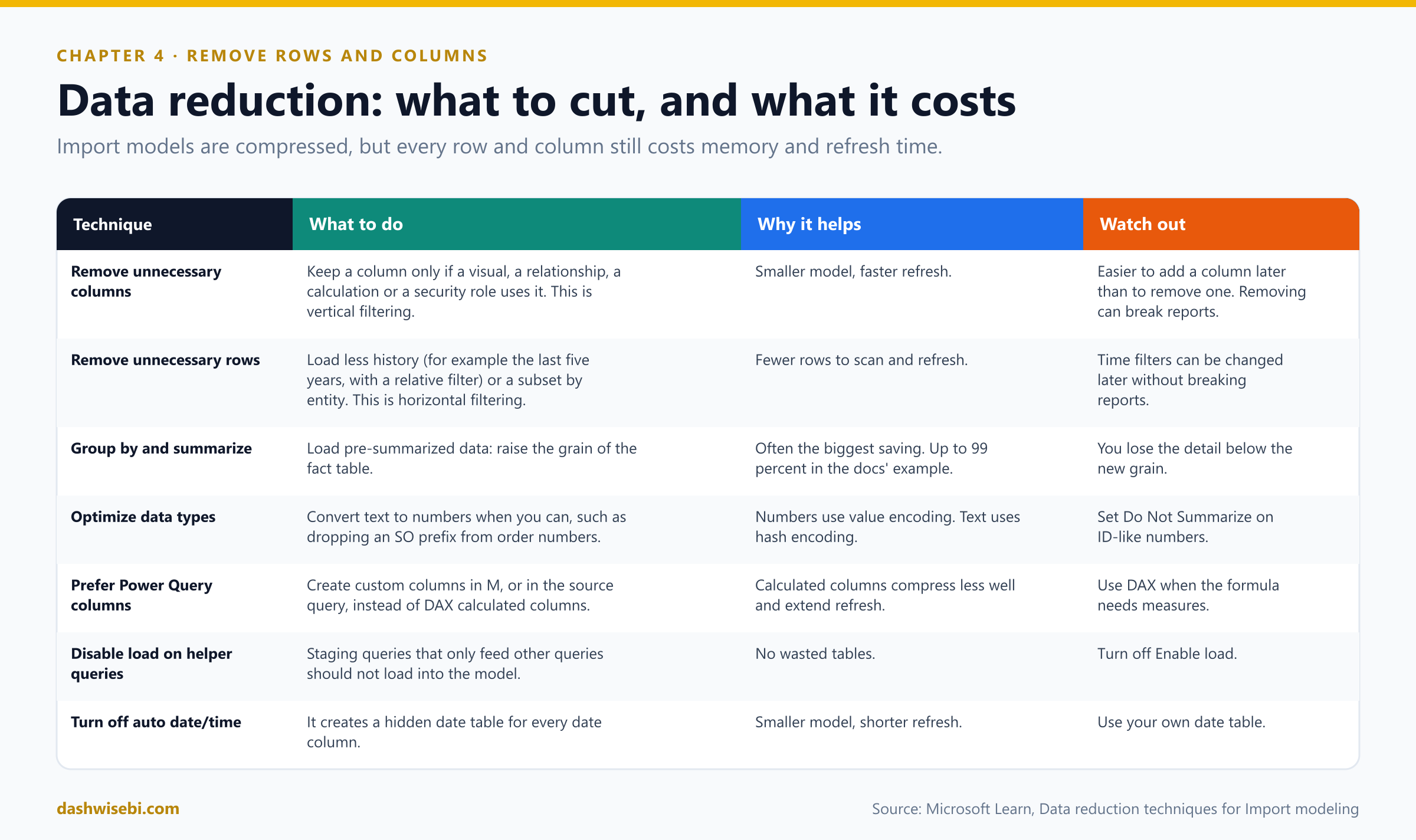
- Vertical filtering (columns): keep a column only if it serves reporting (filter, group, summarize) or model structure (relationships, calculations, security roles, color formatting).
- Horizontal filtering (rows): filter by time (do not load all history by default) or by entity (one region per model, which can also remove the need for row-level security but needs more models and permissions). A time filter can be a Power Query parameter or a relative window, such as the last five years, and changing it later does not break reports.
- Prefer Power Query columns to DAX calculated columns. VertiPaq stores calculated columns less efficiently and builds them after all tables load, so refresh takes longer. Use a DAX calculated column when the formula needs measures or DAX-only functionality.
- Disable load on queries that only feed other queries. Turn off auto date/time, which creates a hidden date table for each date column.
In Power Query, the first two techniques look like this. The relative filter always keeps the last five years, whenever the refresh runs:
let
    Source  = Sql.Database("freshkart-sql", "FreshKart"),
    Lines   = Source{[Schema = "dbo", Item = "OrderLines"]}[Data],

    // Horizontal filtering: only the last five years of history
    Recent  = Table.SelectRows(
                  Lines,
                  each [OrderDate] >= Date.AddYears(Date.From(DateTime.LocalNow()), -5)
              ),

    // Vertical filtering: keep only the columns the model uses
    Slim    = Table.SelectColumns(
                  Recent,
                  {"OrderDate", "StoreKey", "ProductKey", "Qty", "NetAmount", "Cost"}
              )
in
    Slim
Finding what is unused. Open the DAX query view and, in the Data pane, right-click the table and choose Quick queries, Show column statistics to see how each column looks. Use Define all measures in the model to list every measure formula in one place, then search it for the column's name before you remove it.
Three days later, the model is 700 MB and refreshes in twelve minutes. IT sends a thumbs-up, which in IT is a standing ovation.
Exam lens
- Remove columns that serve neither reporting nor model structure. Remove rows by time or by entity.
- Numbers compress better than text. Power Query columns beat DAX calculated columns for size and refresh.
- Hiding is not removing.
- Auto date/time adds hidden tables.
Chapter 5. Rohit again: why is it slow?
The model is smaller, but Rohit's dashboard still takes eight seconds to load. He does not want a theory. He wants a name.
Rohit: Which visual is the problem?
Two tools answer that together. Performance Analyzer tells you where the time goes. DAX query view lets you test why.
Pause and decide. A card shows a DAX query duration of 0.2 seconds, a visual display of 0.1 seconds, and an Other of 4.8 seconds. Where is the problem?
Not in that card's query or drawing. Other is time spent preparing queries, waiting for other visuals to finish, or doing background work. Most visual work shares a single thread, so durations include time spent in the queue. The page probably has too many visuals competing. Reduce the number of visuals, and move detail to a drillthrough page or a tooltip.
Pause and decide. A table visual lists every order line, 100 million rows, until a slicer narrows it. Which duration will be large, and what is the cheapest fix?
Mostly visual display and the DAX query. The default view is unfiltered. Apply the most restrictive filters: for example a Top N filter that caps the rows at more than users would ever read. The experience does not change, but memory and time drop a lot.
Pause and decide. You rewrite a slow measure. How do you compare the old and the new formula safely, without touching the model?
In DAX query view, with DEFINE MEASURE. A query-scoped measure exists only inside the query. Run both versions, compare results and timing, and only then use Update model with changes (or CodeLens) to write the winner back.
Why: Performance Analyzer
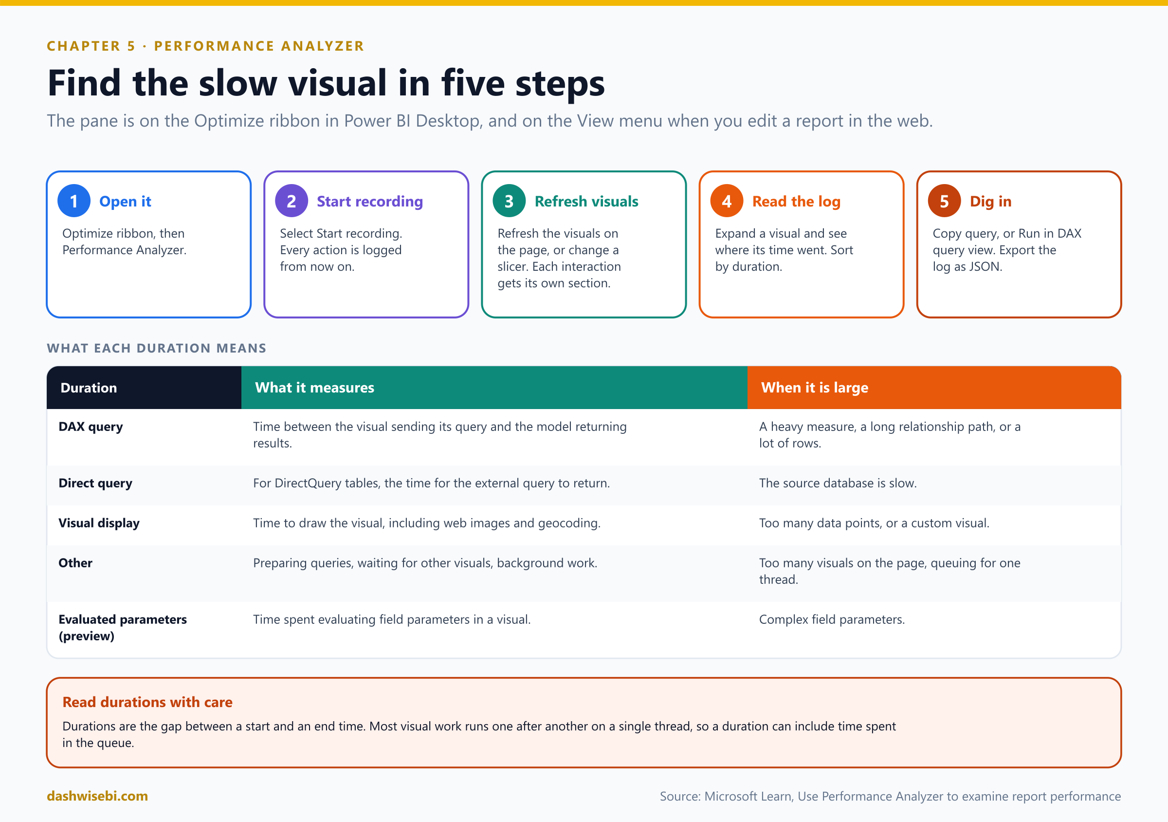
- Find it on the Optimize ribbon in Power BI Desktop, or on the View menu when you edit a report in the web.
- Select Start recording, then Refresh visuals to time every visual on the page. You can also interact (move a slicer) or select Analyze this visual on a single visual. Each interaction gets its own section in the log. Stop ends recording, Clear erases the log, and Export saves a JSON file.
- For each visual you see durations: DAX query, Direct query (DirectQuery tables), Visual display, Other, and Evaluated parameters (preview, for field parameters).
- Expand a visual and select Copy query to get its DAX, or Run in DAX query view (Desktop only) to open it, run it and see the result grid. In the web, copy the query and paste it into DAX query view from the web modeling experience.
Why: DAX query view
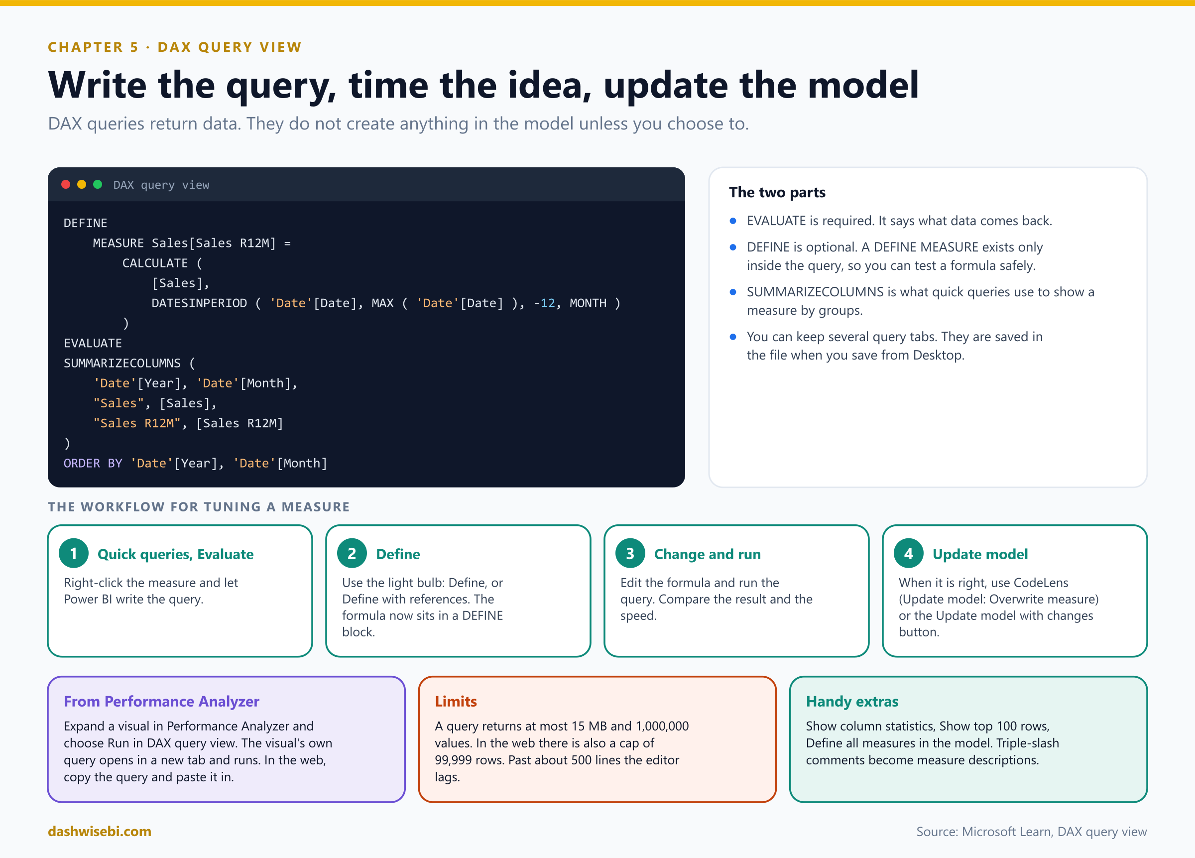
DEFINE
    MEASURE Sales[Sales R12M] =
        CALCULATE (
            [Sales],
            DATESINPERIOD ( 'Date'[Date], MAX ( 'Date'[Date] ), -12, MONTH )
        )
EVALUATE
SUMMARIZECOLUMNS (
    'Date'[Year], 'Date'[Month],
    "Sales", [Sales],
    "Sales R12M", [Sales R12M]
)
ORDER BY 'Date'[Year], 'Date'[Month]- A DAX formula defines a calculation. A DAX query returns data.
EVALUATEis required and says what comes back.DEFINEis optional and can hold query-scoped measures. - Right-click a measure in the Data pane and choose Quick queries: Evaluate, Define and evaluate or Define with references and evaluate. Power BI writes the query for you. Edit it, run it, and when the result is right use CodeLens (Update model: Overwrite measure) or the Update model with changes button.
- Triple-slash (
///) comments above a measure become the measure's description when you update the model. - Limits: a query returns at most 15 MB and 1,000,000 values. In the web there is also a cap of 99,999 rows, and you need write permission on the semantic model. Past about 500 lines the editor lags.
Why: from symptom to suspect
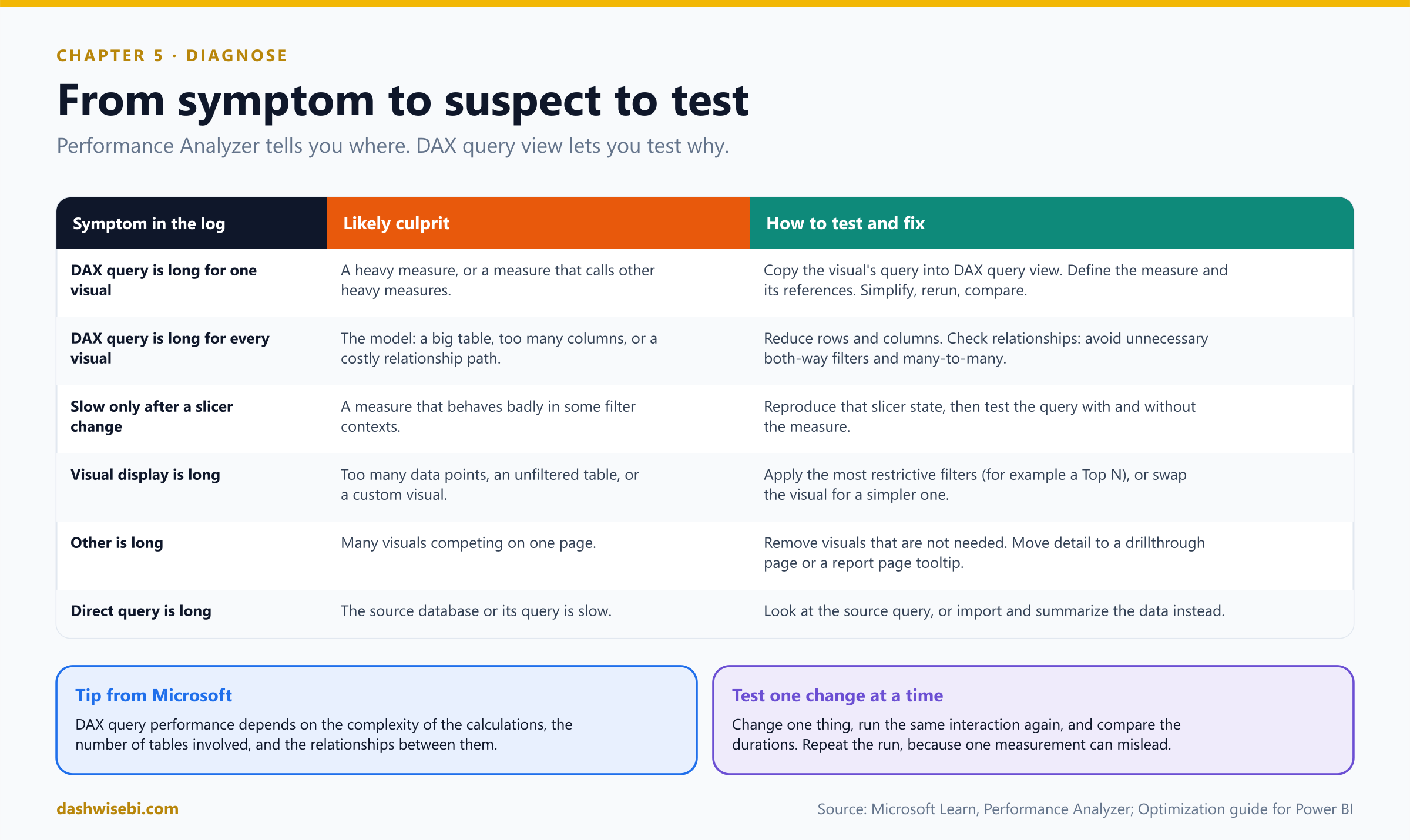
Microsoft's tip is worth memorizing: DAX query performance is affected by the complexity of the calculations, the number of tables involved, and the relationships between them. That is why the same tool tests measures and relationships. Run the visual's query, then change one thing and run it again:
- Measures. Define the measure and the measures it references, simplify, rerun. A common improvement is to replace a
FILTERover a whole fact table with a plain column condition. It usually returns the same result, but it can behave differently if a filter on that column already exists, so confirm in DAX query view:
-- Iterates the whole Sales table row by row
Big Orders Sales =
CALCULATE ( [Sales], FILTER ( Sales, Sales[NetAmount] > 1000 ) )

-- A simple column condition: the engine can use it directly
Big Orders Sales (v2) =
CALCULATE ( [Sales], Sales[NetAmount] > 1000 )- Relationships. Many tables in the filter path, both-way filters and many-to-many relationships (Episode 3) make queries more expensive. If one measure is slow only when it crosses a certain relationship, test it with and without that path.
- Visuals. Limit visuals per page, apply restrictive filters, and use drillthrough pages and report page tooltips for detail. Test custom visuals carefully: a poorly optimized one can slow the entire report.
- Repeat the test. One run can mislead. Run the same interaction a few times and compare like with like.
The log shows it clearly. One matrix, with a rolling-twelve-month measure over an unfiltered 100-million-row detail table, takes 6.5 of the 8 seconds. You give Rohit a name, and he gives you a deadline.
Exam lens
- Performance Analyzer: Optimize ribbon, Start recording, Refresh visuals; durations are DAX query, Direct query, Visual display, Other.
- It exports JSON, and can copy a visual's query or run it in DAX query view.
- DAX query view:
EVALUATE(required) andDEFINE(optional), query-scoped measures, Update model with changes. - Slow queries: look at calculations, tables involved and relationships. Slow visuals: filters, fewer visuals.
Chapter 6. Neha asks: do we need every order line?
It is late. Your own question has been nagging you all day, and you finally say it aloud to the empty room.
You: Nobody looks at individual order lines. Do we really need 120 million of them in an Import model?
The most effective technique to reduce a model's size, according to Microsoft, is to load pre-summarized data: raise the grain of the fact table. The grain is what one row means. Today, one row is one order line. You could make it one row per product, per store, per day.
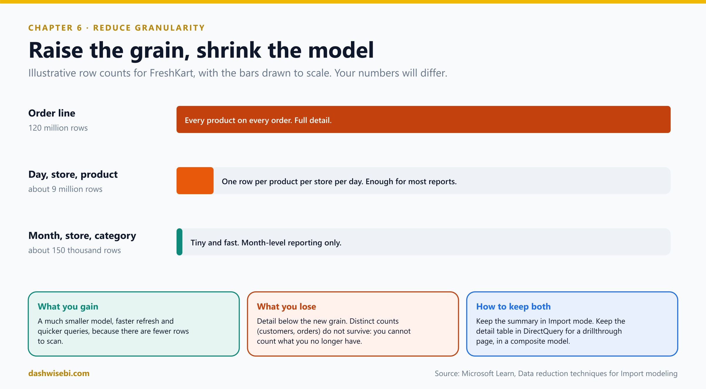
Pause and decide. After summarizing to one row per day, store and product, which of these can you no longer answer: (a) total sales by month, (b) the number of distinct orders per day, (c) sales by store and product category, (d) the basket of one specific order?
(b) and (d). Sums and counts of rows survive summarizing, so (a) and (c) still work. But a distinct count of orders or customers needs the detail you grouped away, and the contents of one order are gone. Decide the grain from your real questions, and keep any count you need as an additive column (for example the number of order lines).
Pause and decide. Managers still want to drill from a summary into the order lines for one store and one day. You do not want 120 million rows in memory. What design keeps both?
A composite model: keep the summarized fact table in Import mode for fast reporting, and keep the detail table in DirectQuery. A drillthrough page filters the detail to a narrow context and retrieves only those rows from the source. Weigh the security and performance implications of DirectQuery before you adopt it.
Pause and decide. The source has an OrderDateTime column with seconds. Reports only ever use the date. What is the smallest change that reduces the model?
Reduce the granularity of the column too: keep only the date (or split date and time and drop the time). Every distinct timestamp is a distinct value to store, so a date has far fewer unique values than a date-time. The same idea, applied to rows, is the summarized fact table.
Why: Group By in Power Query
let
    Source = Sql.Database("freshkart-sql", "FreshKart"),
    Lines  = Source{[Schema = "dbo", Item = "OrderLines"]}[Data],
    Recent = Table.SelectRows(Lines, each [OrderDate] >= #date(2022, 4, 1)),

    // Raise the grain: one row per day, store and product
    Daily  = Table.Group(
        Recent,
        {"OrderDate", "StoreKey", "ProductKey"},
        {
            {"Qty",        each List.Sum([Qty]),        Int64.Type},
            {"NetAmount",  each List.Sum([NetAmount]),  Currency.Type},
            {"Cost",       each List.Sum([Cost]),       Currency.Type},
            {"OrderLines", each Table.RowCount(_),      Int64.Type}
        }
    )
in
Daily- Group By collapses rows that share the same values in the grouping columns and applies an aggregation to the rest. In the Power Query editor use Home, Group By. When the source is a database and the step folds (Episode 2), the database does the grouping and only the small result is loaded.
- The aggregations you keep must be additive: sums and counts. Keep
QtyandNetAmountand compute an average price in a measure asDIVIDE ( [NetAmount], [Qty] ). Never store an average and average it again. - The Microsoft example is dramatic: grouping a sales fact table by date, customer and product, and then by date at month level, could achieve about a 99 percent reduction in model size, but reporting at day level or order-line level is then impossible. The trade-off is the whole story.
- Relationships do not change: the summarized table still relates to Date, Store and Product on the same keys, now with far fewer rows.
The refresh now takes four minutes. The model is 380 MB. The dashboard opens in under two seconds. Rohit says nothing, which, from Rohit, is praise.
Exam lens
- Reduce granularity = Group by and summarize in Power Query, to raise the grain of the fact table.
- It is the most effective size reduction, with a loss of detail. Distinct counts below the new grain are gone.
- Keep detail with a DirectQuery table in a composite model.
The review: nine quick calls
It is the last day of the quarter. Rohit's whole team gathers around your desk and fires questions at you. Answer in your head first, then open each one.
Pause and decide. 1. A fiscal year ends on 30 June. How do you write year to date?
TOTALYTD ( [Sales], 'Date'[Date], "6/30" ): the year_end_date argument, as month/day text.
Pause and decide. 2. A time intelligence function errors out when you give it the date column from the fact table. Why?
The column has gaps. Classic time intelligence needs a complete date column. Use a dedicated, marked date table with no missing dates.
Pause and decide. 3. Stock on hand shows 310 for a product with 120, 100 and 90 on three days. What was wrong, and what are two correct answers?
It summed a semi-additive measure across time. Correct answers: the closing balance (90, with LASTDATE or CLOSINGBALANCEMONTH) or the average (about 103.3, with AVERAGEX).
Pause and decide. 4. The last day of a month has no inventory snapshot, so a closing-balance measure is blank. Fix?
Use LASTNONBLANK or LASTNONBLANKVALUE to fall back to the last date that has data.
Pause and decide. 5. You add a calculation group and a report author cannot drag Sales[NetAmount] into a visual as a sum. Why?
Power BI discourages implicit measures once a calculation group exists, because calculation items apply only to explicit measures. Create an explicit measure instead.
Pause and decide. 6. A calculation item shows a growth percentage as a currency amount. Fix?
Turn on a dynamic format string for that item and return a percentage format.
Pause and decide. 7. Which tool shows how long each visual on a page takes, split into DAX query, visual display and other?
Performance Analyzer: Start recording, then Refresh visuals.
Pause and decide. 8. You want to try a new formula for a measure and compare it with the old one, without changing the model. Which tool and statement?
DAX query view with a DEFINE MEASURE block, then EVALUATE. Update the model only when the result is right.
Pause and decide. 9. The model is too big, and nobody uses order-line detail. Name the technique, and the trade-off.
Group by and summarize (reduce granularity). Big size and refresh savings, in exchange for losing detail below the new grain, including distinct counts.
The cheat sheet
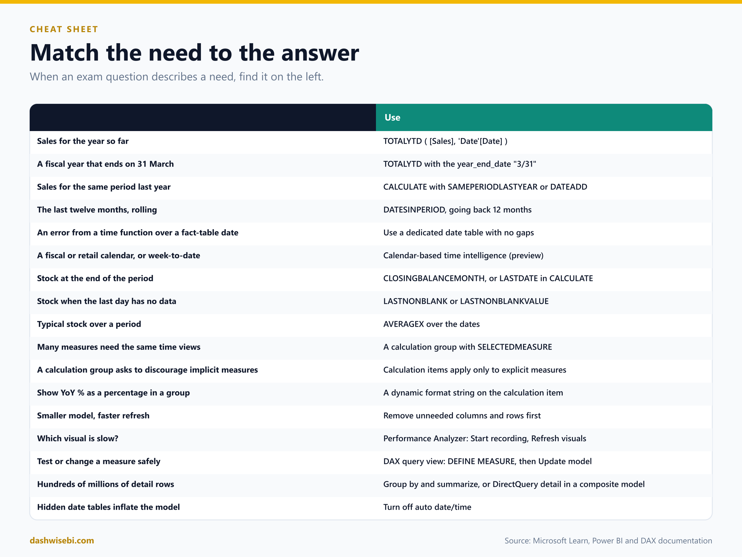
Myth or fact?
- “Time intelligence works on any date column.” Myth. Use a dedicated date table with no gaps.
- “Compare this year's YTD with last year's full total.” Myth. Compare YTD with the prior year's YTD.
- “Auto date/time is free.” Myth. It creates a hidden date table per date column and grows the model.
- “Stock can be summed across days.” Myth. It is semi-additive. Take the last, first or average value.
- “LASTDATE always finds the last stock figure.” Myth. If that day has no data, you get blank. Use LASTNONBLANK.
- “Calculation items apply to every measure and every column.” Myth. Only to explicit measures.
- “Hiding a column shrinks the model.” Myth. Remove it to shrink the model.
- “DAX calculated columns are as efficient as Power Query columns.” Myth. They compress less well and extend refresh.
- “Performance Analyzer shows only DAX time.” Myth. It also shows visual display, Other, and DirectQuery time.
- “A DEFINE MEASURE changes the model.” Myth. It exists only in the query until you update the model.
- “Summarizing to daily keeps distinct counts.” Myth. Distinct counts below the new grain are lost.
Where to go next
- Build the date table from Episode 3, then write
Sales YTD,Sales PYandSales R12M. Put them in a matrix by month and check them against a simple filter. - Create an inventory snapshot table. Show the wrong total with a plain sum, then fix it with
LASTDATE,LASTNONBLANKandAVERAGEX. - Build the Time Calculation group with five items. Add a dynamic format string to YoY %, and try a slicer on the group column.
- Open Performance Analyzer on one of your own reports. Find the slowest visual, copy its query into DAX query view and try to make it faster.
- Take your largest fact table and ask: which columns are unused, and what grain do my reports really need?
- Coming later: single aggregation measures,
CALCULATEfilter patterns, basic statistical functions and quick measures. - Read the sources behind this post: PL-300 study guide, Implement time-based calculations in Power BI, Time intelligence functions (DAX), TOTALYTD, SAMEPERIODLASTYEAR, DATEADD, CLOSINGBALANCEMONTH, LASTNONBLANK, LASTNONBLANKVALUE, Create calculation groups in Power BI, Auto date/time guidance, Data reduction techniques for Import modeling, Optimization guide for Power BI, Use Performance Analyzer to examine report performance and DAX query view.
Keep reading
PL-300 Episode 6: Copilot, Visual Calculations & Analytics
PL-300 as a five-day story: Copilot, visual calculations, grouping and clustering, AI visuals, Analyze, anomalies, reference lines and forecasts.
PL-300 Episode 3: Design the Data Model
PL-300 Episode 3: star, snowflake and galaxy schemas, properties, relationships, role-playing dimensions, date tables, calculated columns and tables, with M and DAX.