Spark Basics

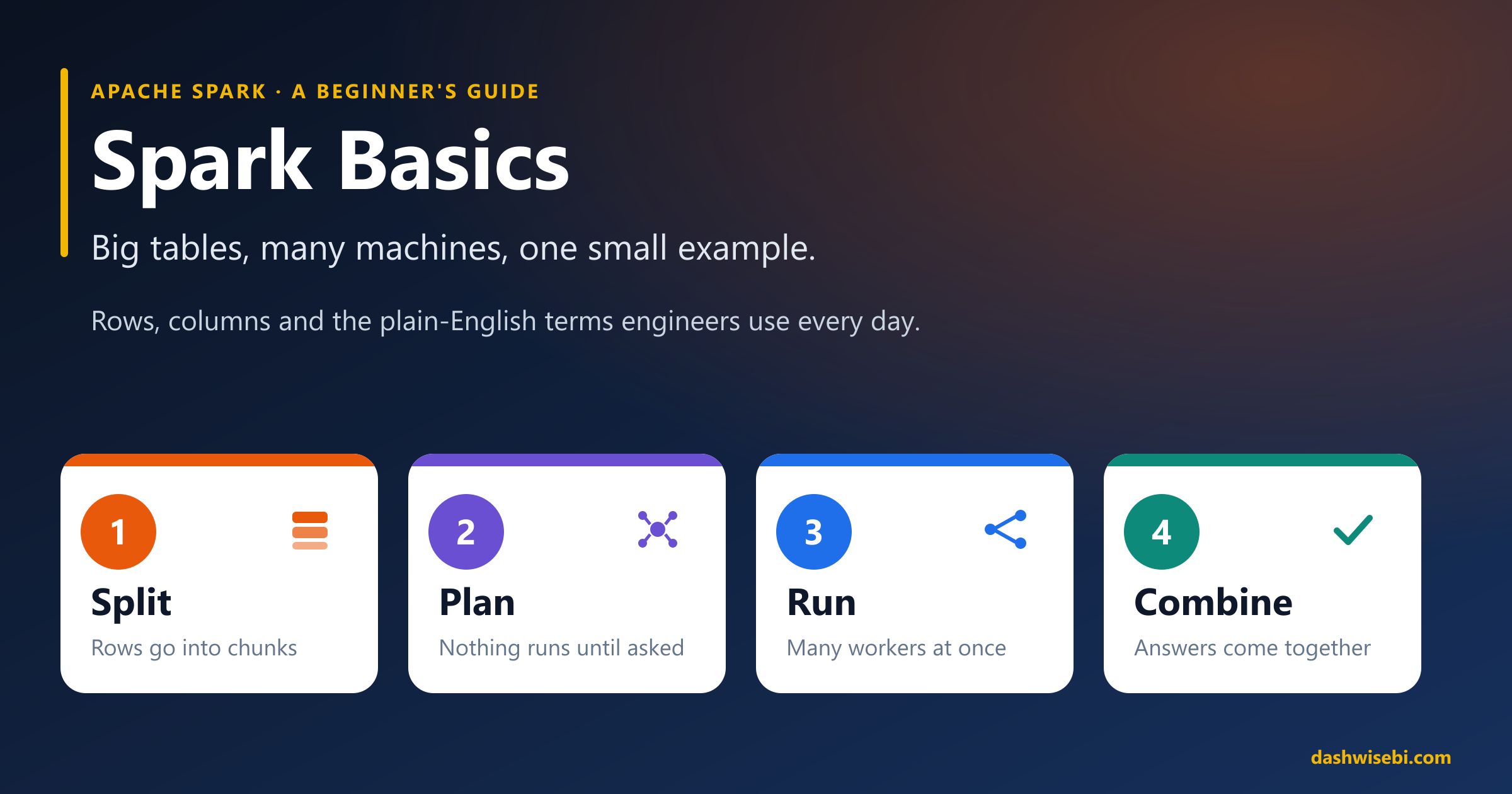
Apache Spark has a reputation for being hard. It is not, once you see what it is really doing. Spark takes a table that is too big for one computer, cuts it into pieces, hands the pieces to many computers, and combines their answers.

That is the whole idea. Everything else, the driver, executors, partitions, shuffles and the rest of the vocabulary, is just a name for one step of that story.

This post explains Spark in plain English. Every idea is shown on the same small table of orders, so you can follow the rows and columns from the first section to the last. The facts come from the official Apache Spark documentation, and the sources are listed at the end.

What is Spark, in one sentence?

The Spark website describes Apache Spark as a multi-language engine for data engineering, data science and machine learning, running on a single machine or on a cluster. You can write Spark programs in Python, SQL, Scala, Java or R.

A cluster is just a group of computers working together. The word you will hear most in the rest of this post is distributed, which simply means "spread across many computers".

If you use Microsoft Fabric, you are already using Spark every time you run a notebook. Our DP-700 post on Fabric workspace settings shows where its compute is configured.

Our example: one small table

Here is the table we will use everywhere. It holds orders from a shop, with five columns and eight rows.

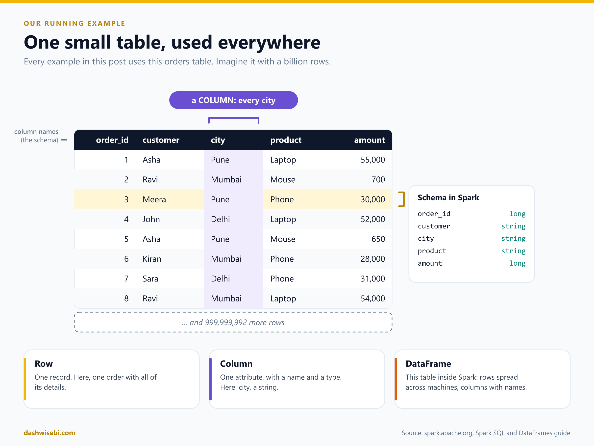
• A row is one record. Row 3 is one order: Meera bought a phone in Pune for 30,000.
• A column is one kind of fact, with a name and a type. The city column holds a text value (a string) for every order.
• The column names and types together are the schema.
• In Spark, a table like this is called a DataFrame. The Spark guide defines it as a dataset organised into named columns, much like a table in a relational database.

Eight rows is easy. Now imagine the same five columns with a billion rows. That is where the trouble starts.

Why Spark exists: the table is too big

Picture grading exam papers. One teacher can grade 10 papers quickly. Give that teacher a million papers and it takes forever. Give each of 100 teachers 10,000 papers, let them work at the same time, and then add up the marks, and the job is done far sooner. Spark does exactly this with rows.

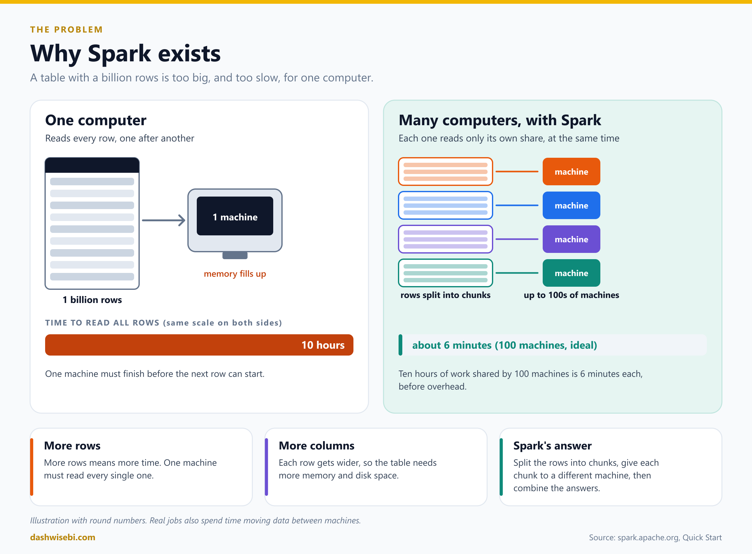
Two things make a big table hard for a single machine:

• More rows means more time. One machine must read every row, one after another. If reading a billion rows takes 10 hours, spreading them over 100 machines that each read a hundredth of the rows takes about 6 minutes in the ideal case. The numbers here are round figures for illustration, and real jobs lose some time moving data between machines.
• More columns means more memory. Every row gets wider, so the whole table needs more memory and disk space than one machine may have.

Spark's answer is to split the table by rows, so many machines can work at once, and to read only the columns you need, so each machine does less. We will see both ideas in action below.

The Spark Quick Start makes the same point: the commands you try on a tiny file work unchanged on very large datasets spread across tens or hundreds of machines. The Spark homepage also says data scientists can explore petabyte-scale data without having to cut it down to a sample first.

Meet the team: driver, executors and the cluster manager

A Spark job has a few characters. It helps to think of a small company.

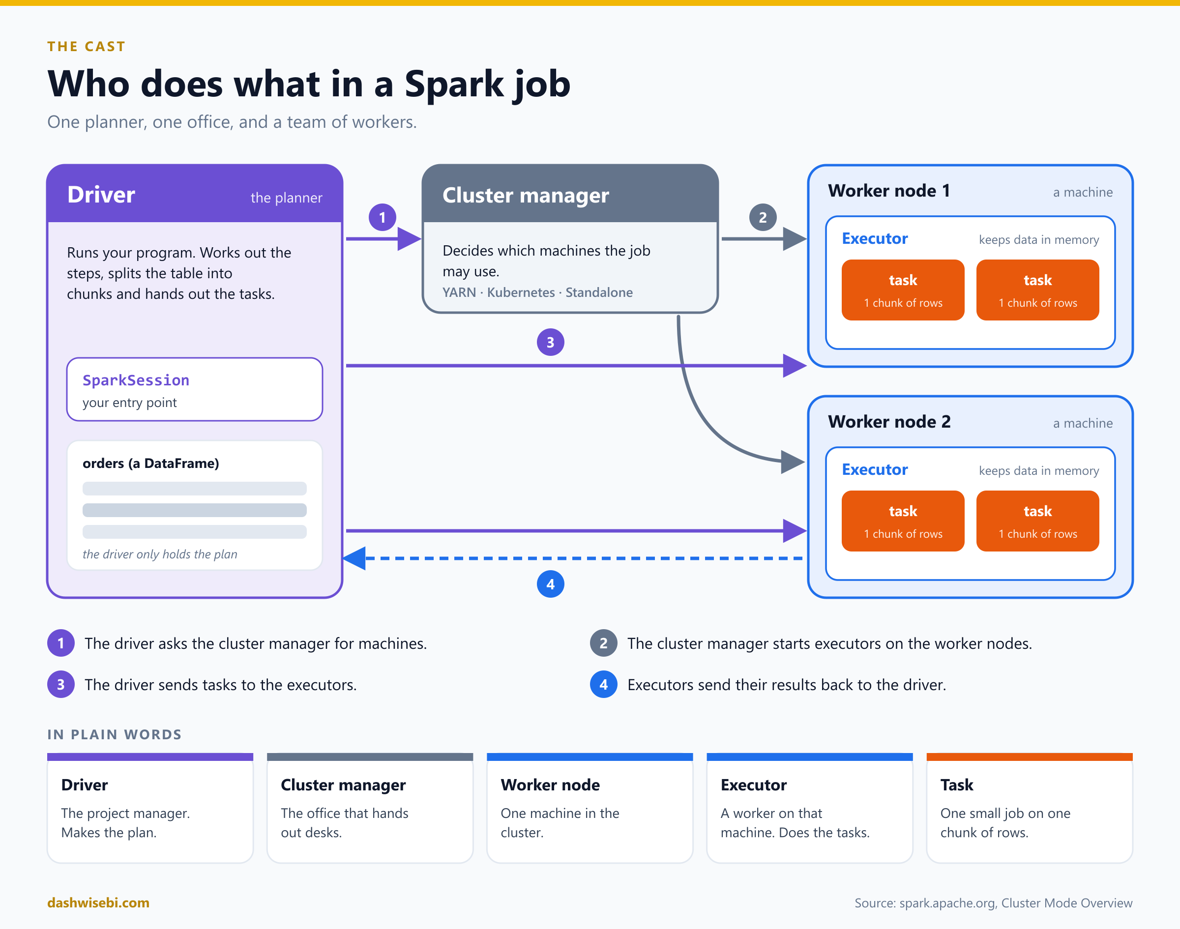
• The driver is the project manager. It runs your program, works out the steps, and splits the table into chunks. Your code reaches it through the SparkSession, the entry point you create at the start of every Spark program.
• The cluster manager is the office that hands out desks. It decides which machines the job may use. Spark works with its own Standalone manager, with YARN and with Kubernetes.
• A worker node is one machine in the cluster.
• An executor is a worker process on that machine. It runs the tasks it is given and keeps data in memory between them. Each application gets its own executors.
• A task is one small piece of work on one chunk of rows.

The order of events is simple. The driver asks the cluster manager for machines, the cluster manager starts executors, the driver sends tasks to the executors, and the executors send the results back. The driver never holds the whole table. It only holds the plan.

The whole bundle, your driver program plus its executors, is called a Spark application.

Splitting the rows: partitions

To share the work, Spark cuts the table into chunks called partitions. Each partition is a set of rows, and each one is handled by one task.

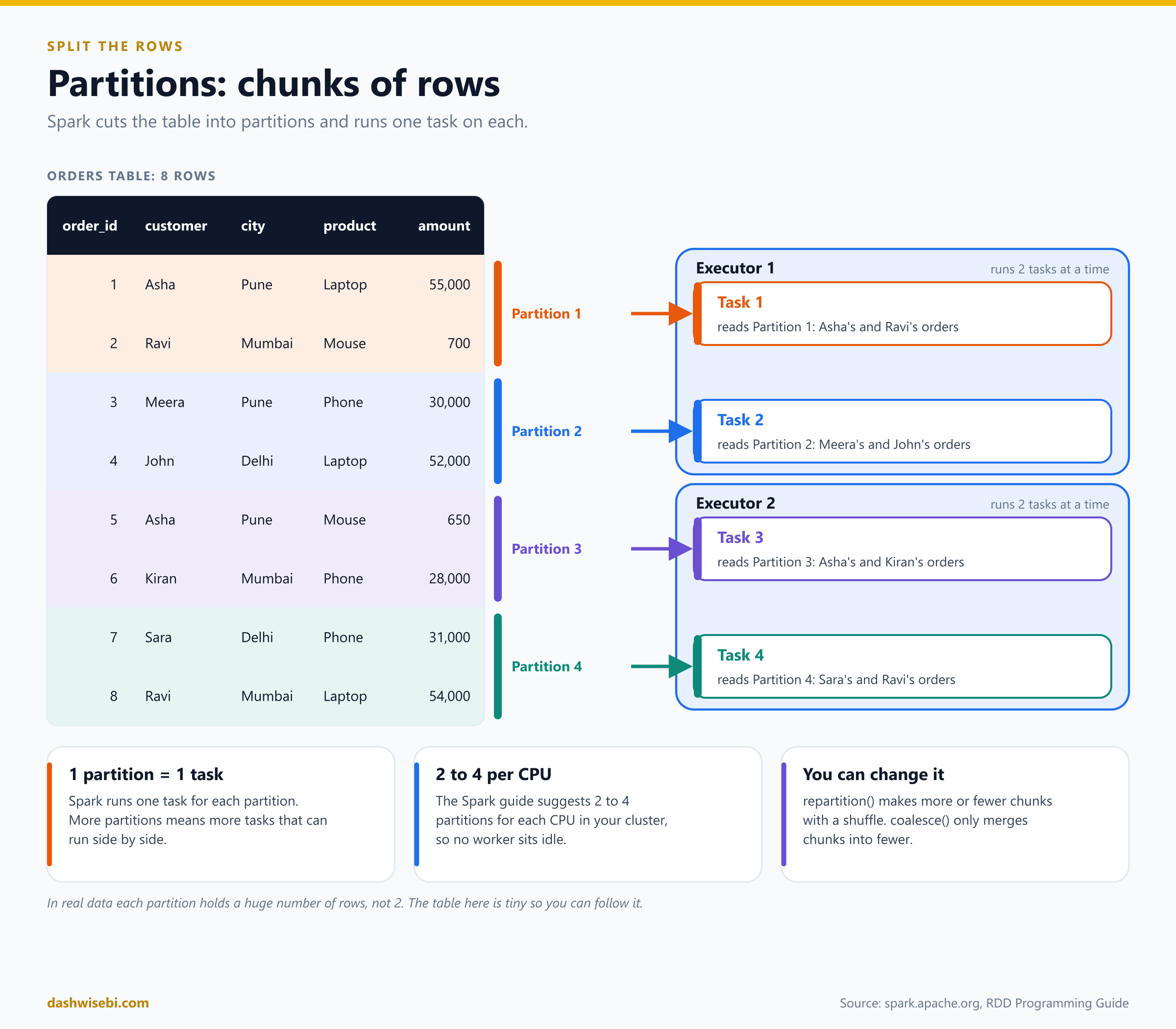
With our eight rows, imagine Spark makes four partitions of two rows each. Partition 1 holds orders 1 and 2, partition 2 holds orders 3 and 4, and so on. Executor 1 runs tasks 1 and 2 while executor 2 runs tasks 3 and 4, all at the same time.

• Spark runs one task for each partition.
• The Spark guide suggests about 2 to 4 partitions for each CPU in your cluster. Fewer than that and some workers sit idle.
• You can change the count with repartition(), which reshuffles rows into more or fewer partitions, or coalesce(), which merges partitions into fewer.

In real data each partition holds a huge number of rows. This is how a billion-row table becomes thousands of small, independent jobs.

Plan first, run later: transformations and actions

Here is a surprise for beginners. When you write a Spark step, nothing happens. Spark just writes the step down. This is called lazy evaluation.

Steps come in two kinds:

• A transformation builds the plan: filter, select, withColumn, groupBy, join. It returns a new table description and does no work.
• An action asks for a result: show, count, collect, write. Only now does Spark run the plan on the cluster.

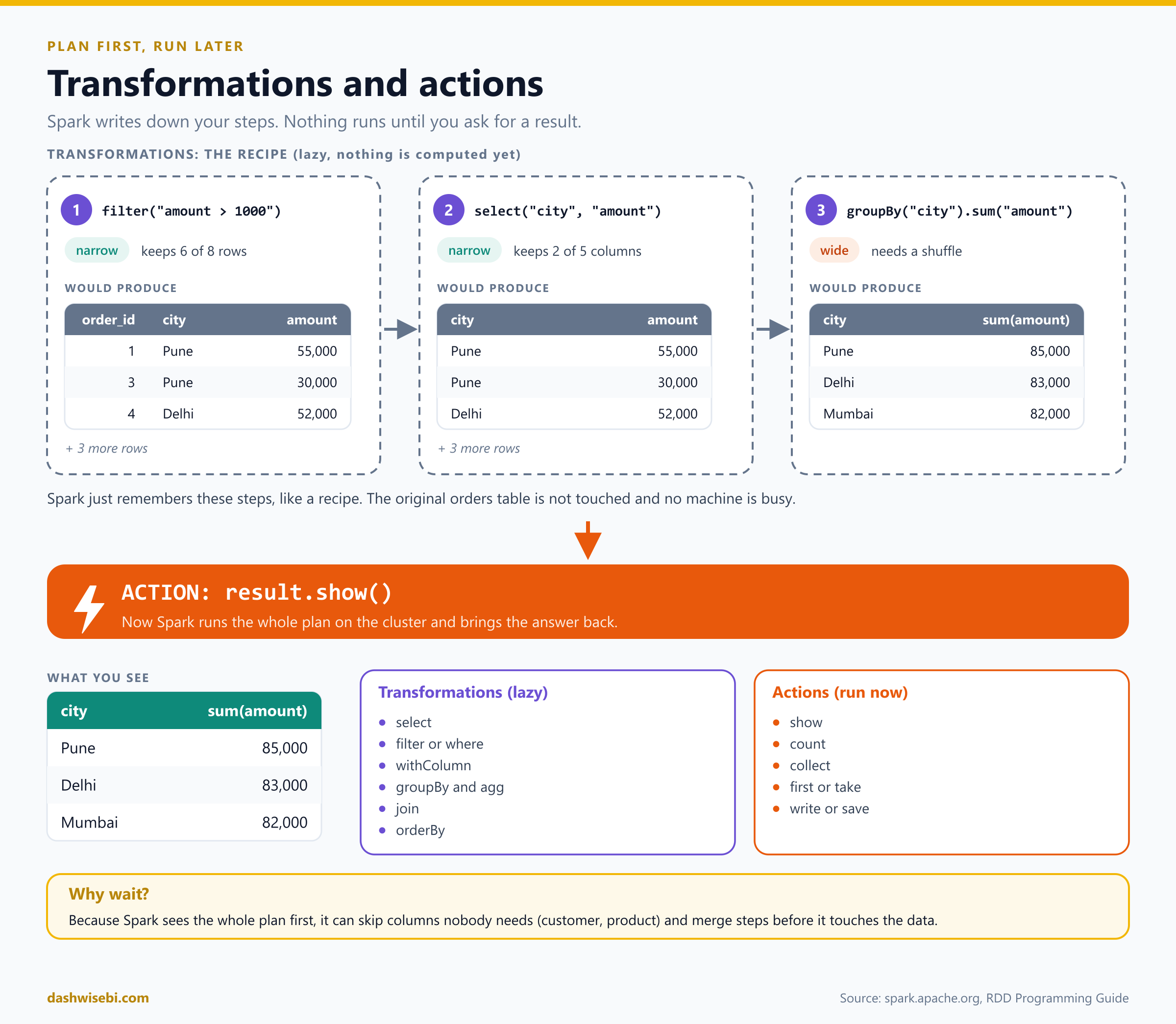
Here is our table going through a plan:

big_orders = orders.filter("amount > 1000")      # transformation: plan only
slim       = big_orders.select("city", "amount")  # transformation: plan only
totals     = slim.groupBy("city").sum("amount")   # transformation: plan only

totals.show()                                     # ACTION: Spark runs everything now

The Spark guide gives a good picture of this: a file you "load" is really just a pointer until an action needs an answer. The reason for waiting is practical. Because Spark sees your whole plan first, it can skip columns nobody needs (here, customer and product) and combine steps before it touches any data.

Transformations also come in two flavours. A narrow transformation, like filter or select, works on each row where it already is. A wide transformation, like groupBy or join, needs rows from different places to meet. That meeting is the next idea.

Under the hood: job, stage, task and shuffle

Let us follow one action on our table: add up the amount for each city.

orders.groupBy("city").sum("amount").show()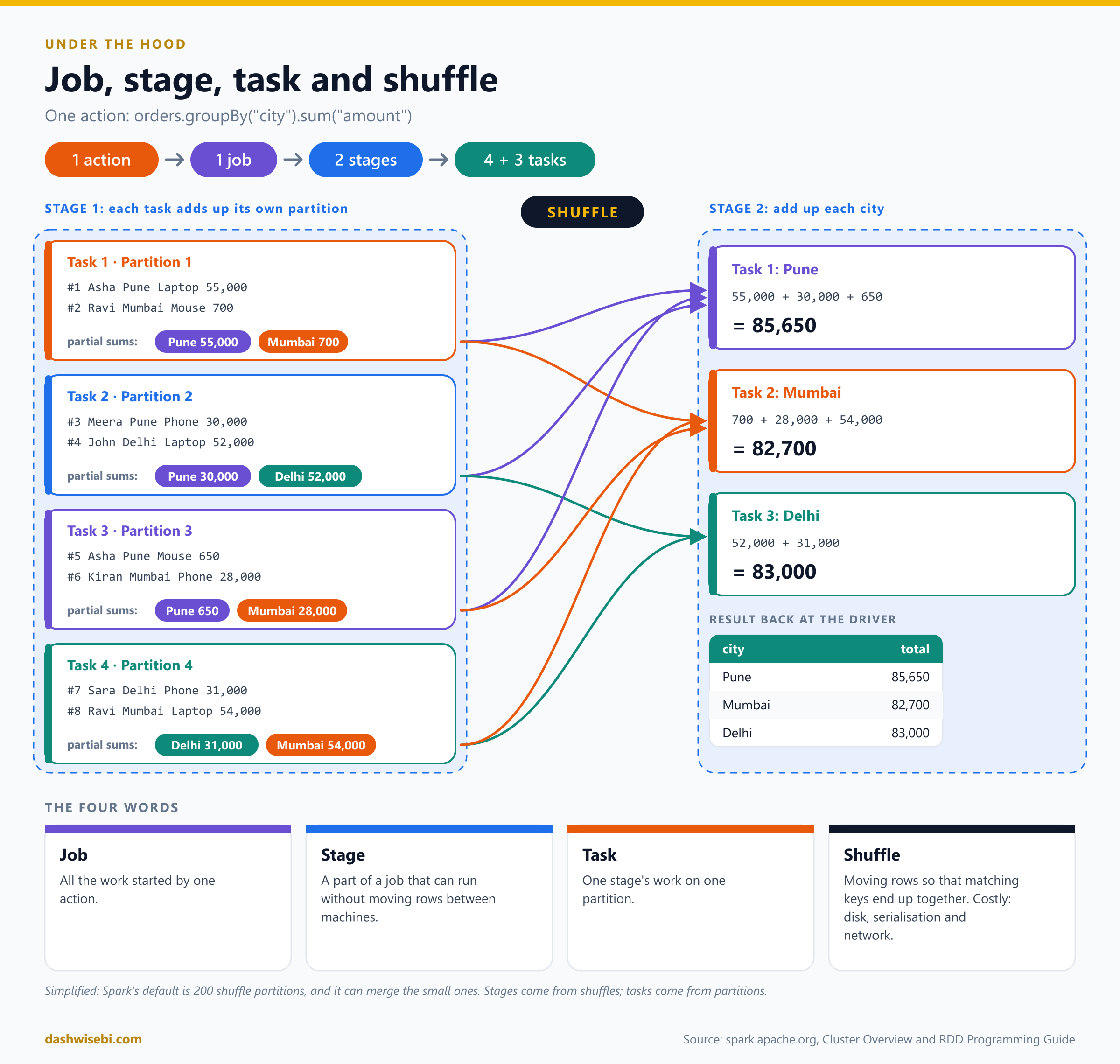

Here is what Spark does:

1. Stage 1. Four tasks run, one per partition. Each task adds up the orders it holds, city by city. Task 1 finds Pune 55,000 and Mumbai 700. Task 2 finds Pune 30,000 and Delhi 52,000. The other two do the same for their rows.
2. The shuffle. The partial totals now sit on different machines, but the answer for Pune needs all the Pune pieces together. So Spark sends every Pune subtotal to one place, every Mumbai subtotal to another, and every Delhi subtotal to a third.
3. Stage 2. Three tasks run, one per city, and add up the pieces they received. Pune: 55,000 + 30,000 + 650 = 85,650. Mumbai: 700 + 28,000 + 54,000 = 82,700. Delhi: 52,000 + 31,000 = 83,000.
4. The three totals go back to the driver, which shows them to you.

That is the whole vocabulary in one example:

• A job is all the work started by one action. Here the show() started one job.
• A stage is a part of a job that can run without moving rows between machines. A shuffle splits a job into stages, which is why this job has two.
• A task is one stage's work on one partition. This job ran 4 + 3 tasks.
• A shuffle is Spark's way of regrouping data across machines.

The shuffle is the expensive part. The Spark guide explains that it involves disk reads and writes, data serialisation and network transfers, which is why engineers try to keep shuffles to a minimum. Operations that cause one include repartition, groupBy-style aggregations, and join.

One note on the picture: it is simplified. Spark's default is 200 shuffle partitions, not three, and it can merge the small ones. Spark also adds up inside each partition first, as our stage 1 does, so less data has to travel.

Why Spark loves columns: reading less

So far we have used rows to explain how Spark goes wide. Columns explain how it reads less.

Imagine the query SELECT SUM(amount) FROM orders. It needs one column out of five.

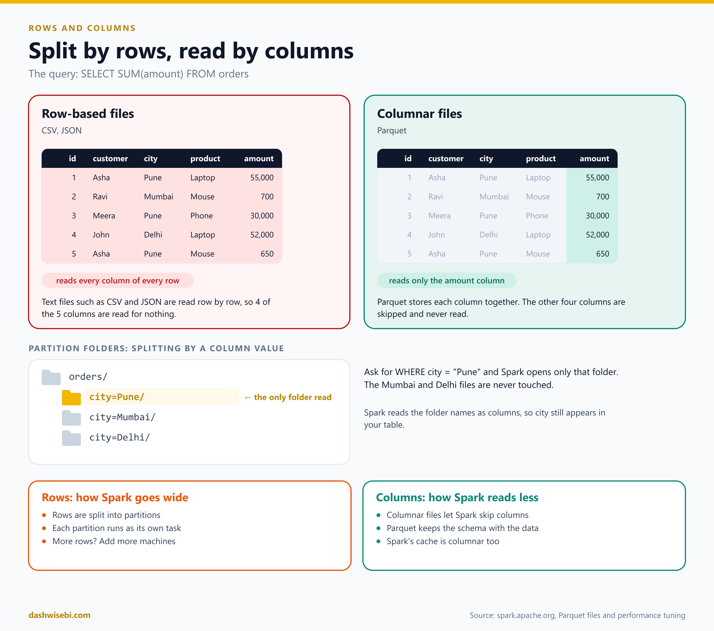
• With CSV or JSON files, data is stored row by row. To get at the amount of each row, the machine still reads the customer, city and product too. Four of the five columns are read for nothing.
• With Parquet, a columnar format that the Spark docs describe in detail, each column is stored together. Spark can read only the amount column and ignore the other four. Parquet files also carry their schema with them, so the column names and types are never lost.

With a billion rows, skipping four columns out of five is a huge saving in disk and network traffic.

There is a second trick. You can store the table in folders by a column value, for example city=Pune/, city=Mumbai/ and city=Delhi/. Ask for orders where the city is Pune, and Spark opens only that folder. The other files are never touched. Spark reads the folder names back as a column, so city still shows up in your table.

Spark applies the same idea in memory. When you cache a table (more on that below), Spark keeps it in a columnar format and scans only the columns a query needs.

Put together: rows are how Spark splits the work, and columns are how Spark avoids work.

Everyday moves on a table

Most of a data engineer's day is a handful of moves. Here they are on our orders table, with the result of each.

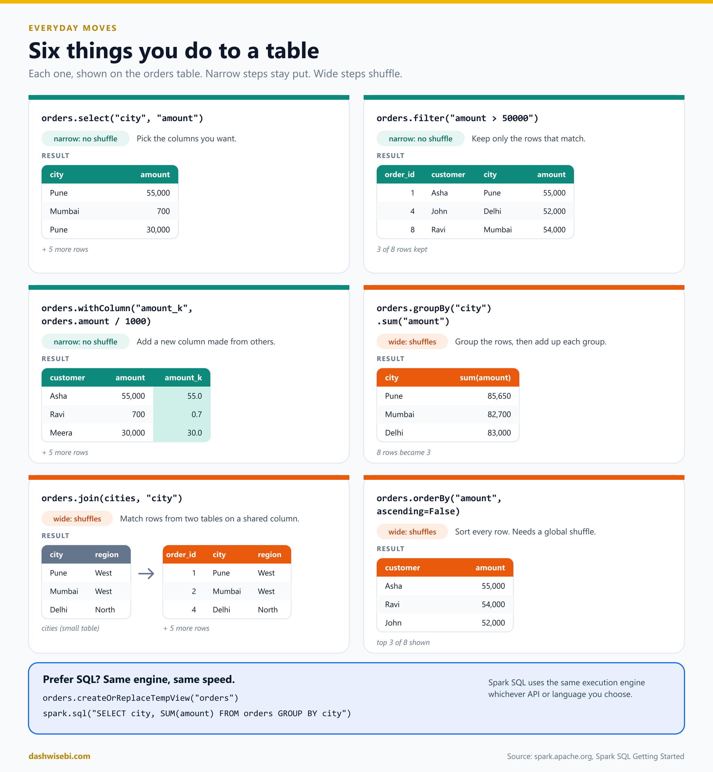
orders.select("city", "amount")                 # pick columns
orders.filter("amount > 50000")                 # keep matching rows
orders.withColumn("amount_k", orders.amount / 1000)  # add a column
orders.groupBy("city").sum("amount")            # add up each group
orders.join(cities, "city")                     # combine two tables
orders.orderBy("amount", ascending=False)       # sort

The first three are narrow, so they stay where the data is. The last three are wide and cause a shuffle, because they need rows from different places to meet.

If you prefer SQL, you can use it on the same data. Register the table as a temporary view and query it:

orders.createOrReplaceTempView("orders")
spark.sql("SELECT city, SUM(amount) AS total FROM orders GROUP BY city").show()

The Spark documentation notes that Spark SQL uses the same execution engine whichever API or language you choose, so this is not slower than the DataFrame version.

Making it fast: cache, broadcast and skew

Once the basics work, three ideas come up again and again in real projects.

1. Cache what you reuse

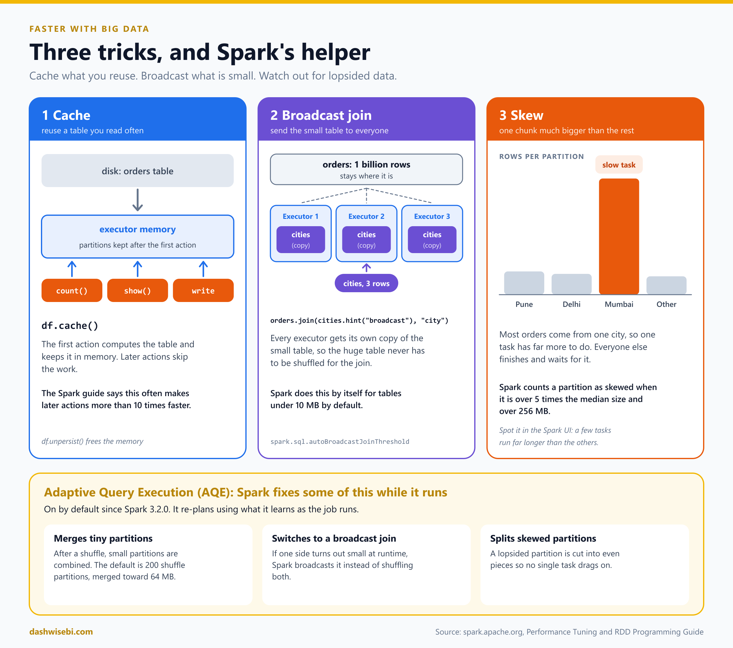
If you use the same table several times, Spark would normally rebuild it each time. orders.cache() tells Spark to keep the partitions in memory the first time they are computed, so later actions reuse them. The Spark guide says this often makes later actions more than ten times faster. Because Spark is lazy, the caching really happens at the first action. When you are finished, unpersist() frees the memory.

2. Broadcast what is small

Suppose you join the huge orders table to a tiny cities table that lists each city's region. Shuffling a billion rows just to match three city names would be wasteful. Instead Spark can broadcast the small table, sending a full copy to every executor. Each executor then joins its own rows locally, and the big table never moves.

orders.join(cities.hint("broadcast"), "city")

Spark does this on its own for tables under about 10 MB by default, and the hint forces it.

3. Watch out for skew

Skew means the data is lopsided. If most orders come from Mumbai, the Mumbai partition has far more rows than the others, so one task takes much longer while the rest sit finished and waiting. Spark treats a partition as skewed when it is more than five times the median size and larger than 256 MB.

Spark can help: Adaptive Query Execution

Spark has a helper called Adaptive Query Execution (AQE). It adjusts the plan while the job runs, using what it learns. It merges tiny partitions after a shuffle (merging toward 64 MB), switches a join to a broadcast join when one side turns out to be small, and splits skewed partitions into even pieces. AQE has been on by default since Spark 3.2.0, and the Spark homepage says it speeds up TPC-DS queries by up to 8 times.

What if a machine fails?

With hundreds of machines, one will eventually fail. Spark is built for that. The word resilient in "resilient distributed dataset" means that if a partition is lost, Spark can rebuild it by replaying the steps that created it. Those remembered steps are called the lineage. The same holds for cached data: if a cached partition is lost, Spark recomputes it. You do not have to start the whole job again.

Where to look when something is slow: the Spark UI

Every running application serves a web page, by default on port 4040 of the driver, called the Spark UI. It is the first place data engineers look when a job is slow.

• Jobs: every job, with status, duration and a timeline.
• Stages: the stages of each job and the metrics for every task, including shuffle read and write and spill to disk.
• Storage: what you have cached, and how big it is.
• Executors: each executor's memory, cores, tasks and time spent in garbage collection.
• SQL: the plan behind each DataFrame or SQL query.

To spot skew, open a stage and compare the task durations. If a few tasks run far longer or read far more data than the rest, the data is lopsided.

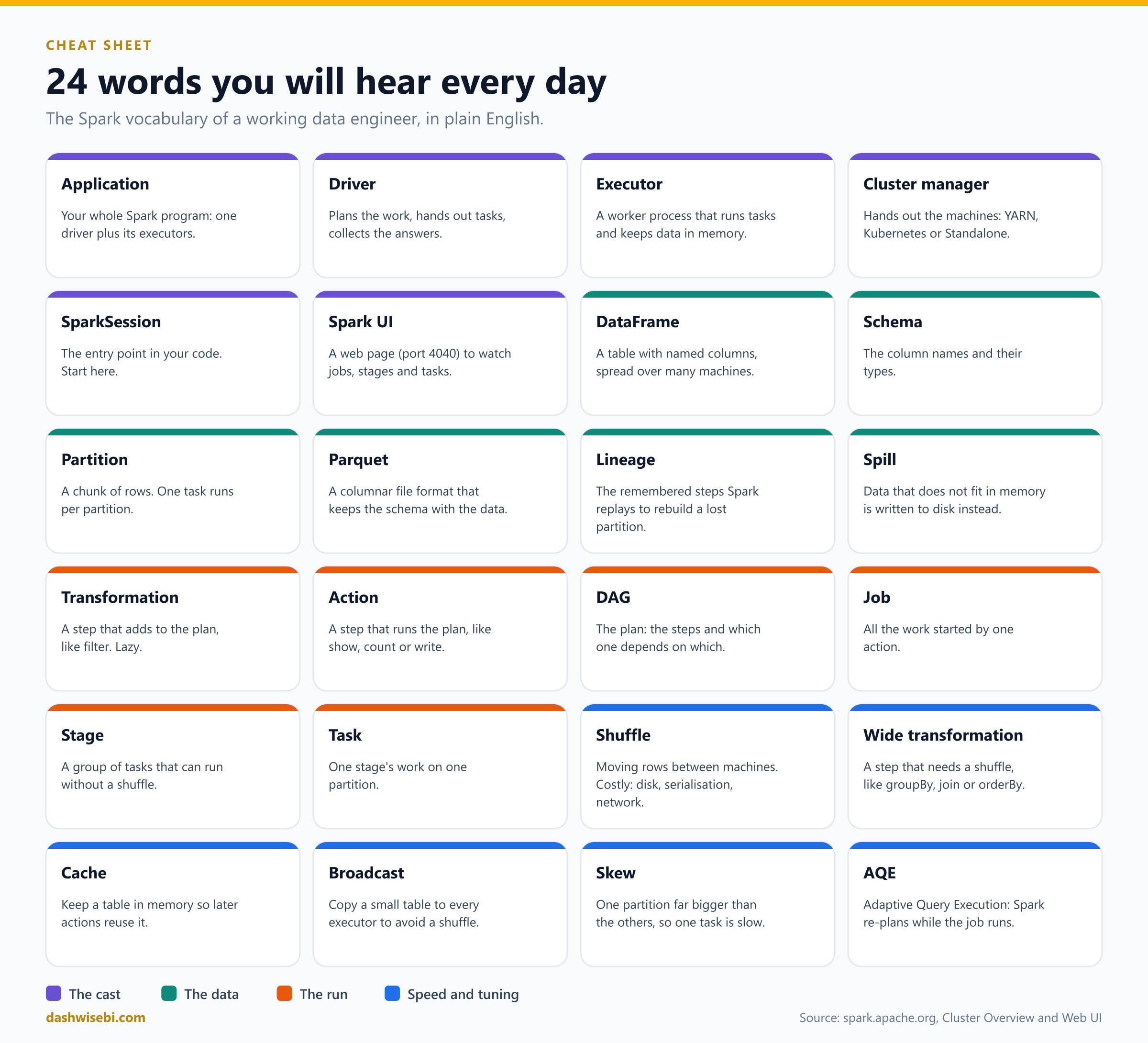
24 words you will hear every day

Putting it all together

Here is a complete small program, using everything above. It reads the orders table from Parquet, keeps the big orders, adds them up by city and shows the result.

from pyspark.sql import SparkSession

spark = SparkSession.builder.appName("orders-demo").getOrCreate()

orders = spark.read.parquet("orders.parquet")        # Spark reads the schema, not the rows

totals = (
    orders
    .filter("amount > 1000")                         # narrow: runs where the data is
    .groupBy("city")                                 # wide: causes a shuffle
    .sum("amount")
)

totals.show()                                        # the action: the plan runs now

On our eight rows, the output looks like this (the row order may differ):

+------+-----------+
|  city|sum(amount)|
+------+-----------+
|  Pune|      85000|
| Delhi|      83000|
|Mumbai|      82000|
+------+-----------+

On a billion rows the code is exactly the same. Only the work behind it changes: more partitions, more tasks, more executors.

The short version

• Rows are split. Spark cuts a big table into partitions and runs one task on each, on many machines at once. That is why it scales to a billion rows.
• Columns are skipped. With columnar files such as Parquet, Spark reads only the columns the query needs.
• Nothing runs until you ask. Transformations build a plan, and an action runs it, so Spark can optimise first.
• Shuffles are the cost. Narrow steps are cheap and wide steps move data, so keep wide steps few.
• Reuse and shrink. Cache what you reuse, broadcast what is small, and let AQE handle the rest.

One honest caveat: Spark is built for large tables. The Spark Quick Start itself says it may seem silly to use Spark on a 100-line file. If your data fits comfortably on one machine, a simpler tool may be quicker, and Spark's overhead only pays off when the table is big.

References from the official Spark site

• Apache Spark homepage
• Quick Start: your first DataFrame, caching, and Spark on large datasets
• Cluster Mode Overview: the driver, executors, cluster manager and the glossary of job, stage and task
• RDD Programming Guide: partitions, lazy transformations and actions, shuffles, caching and broadcast variables
• Spark SQL, DataFrames and Datasets Guide
• Spark SQL Getting Started: SparkSession, DataFrame operations and SQL queries
• Parquet files: columnar storage, schema and partition discovery
• Performance Tuning: caching, shuffle partitions, broadcast joins and Adaptive Query Execution
• Web UI: the tabs of the Spark UI